Defining Functions on SubDomains

In many contexts, fields are required over only a subset of the computational Grid. In Devito, such fields can be implemented via the Functions on SubDomains API, allocating arrays only over the required region of the Grid, thereby reducing memory consumption. This functionality is seamlessly compatible with MPI, as with any other Devito object, and these arrays are aligned with the domain decomposition under the hood.

We will begin with some necessary imports.

import matplotlib.pyplot as plt
import matplotlib.animation as animation
import numpy as np

from IPython.display import HTML

from devito import SubDomain, Grid, Function, Eq, Operator, \
    SparseFunction, ConditionalDimension, TimeFunction, solve, \
    TensorTimeFunction, VectorTimeFunction, diag, grad, div
from examples.seismic import TimeAxis, RickerSource, Model, Receiver

Basic usage

As usual, we define a subdomain template by subclassing SubDomain and overriding the define method. The 'middle' subdomain we have defined in this case excludes two points from each side of the domain in each dimension.

class Middle(SubDomain):
    name = 'middle'

    def define(self, dimensions):
        return {d: ('middle', 2, 2) for d in dimensions}

We then create a Grid, followed by an instance of Middle. We can then use this subdomain as the computational grid when defining a Function. For comparison, we also create a Function defined on a Grid.

grid0 = Grid(shape=(11, 11), extent=(10., 10.))

middle = Middle(grid=grid0)

f = Function(name='f', grid=middle)  # Define Function on SubDomain
g = Function(name='g', grid=grid0)

Inspecting the shape of f, it is apparent that it is smaller than the Grid on which middle is defined. Instead, its shape is that of middle.

f.shape

(7, 7)

Furthermore, f has the dimensions of the SubDomain rather than the Grid.

f.dimensions

(ix, iy)

By contrast, when inspecting g, we observe that its shape and dimensions match those of the Grid.

g.shape

(11, 11)

g.dimensions

(x, y)

To contrast the behaviour of a Function defined on a SubDomain to one defined on a Grid, we implement a trivial Operator, setting both f and g equal to one within the SubDomain middle.

#NBVAL_IGNORE_OUTPUT
eq_f = Eq(f, 1)
eq_g = Eq(g, 1, subdomain=middle)

Operator([eq_f, eq_g])()

NUMA domain count autodetection failed
Operator `Kernel` ran in 0.01 s

PerformanceSummary([(PerfKey(name='section0', rank=None),
                     PerfEntry(time=0.000196, gflopss=0.0, gpointss=0.0, oi=0.0, ops=0, itershapes=[]))])

Note that if there is only one SubDomain on which Functions are defined present in the Eq expressions, Devito will automatically infer the subdomain kwarg if none is supplied. If multiple SubDomains are used to define Functions, but no subdomain is specified in Eq, then an error will be thrown. Inspecting eq_f, we see that the SubDomain is inferred:

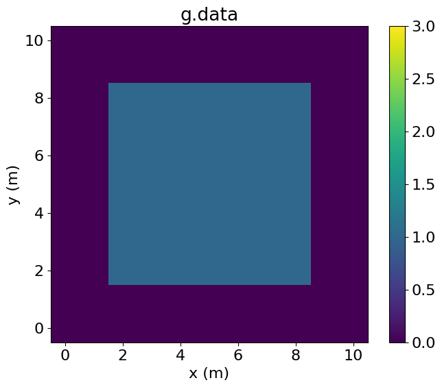
eq_f.subdomain

Middle[middle(ix, iy)]

Examining f.data, we see that it has been entirely set to one by the Operator. By contrast, g.data is only set to one in the central region.

#NBVAL_IGNORE_OUTPUT
plt.imshow(f.data.T, vmin=0, vmax=3, origin='lower', extent=(1.5, 8.5, 1.5, 8.5))
plt.colorbar()
plt.title("f.data")
plt.xlabel("x (m)")
plt.ylabel("y (m)")
plt.xlim(-0.5, 10.5)
plt.ylim(-0.5, 10.5)
plt.show()

plt.imshow(g.data.T, vmin=0, vmax=3, origin='lower', extent=(-0.5, 10.5, -0.5, 10.5))
plt.colorbar()
plt.title("g.data")
plt.xlabel("x (m)")
plt.ylabel("y (m)")
plt.show()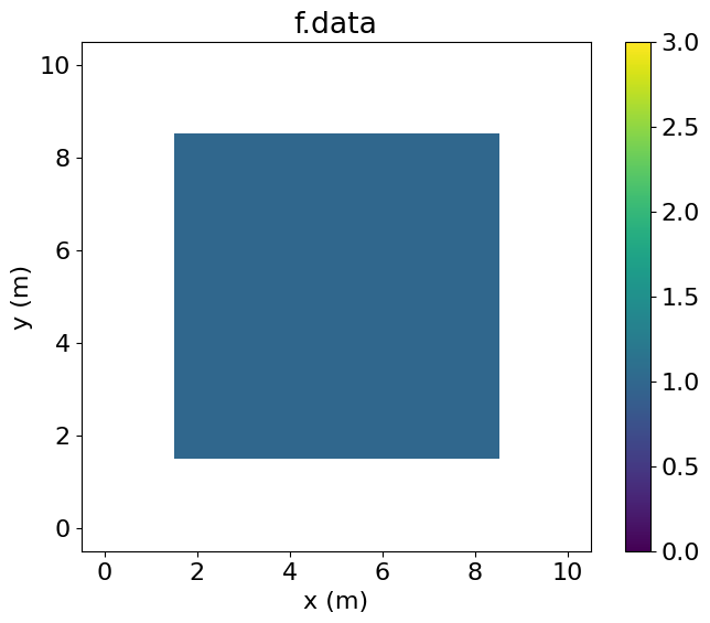

When operating on a Function defined on a SubDomain, Devito keeps track of the alignment of the fields relative to the base Grid. As such, we can perform operations combining Functions defined on SubDomains with those defined on the Grid. For example, we can add f to g as follows:

#NBVAL_IGNORE_OUTPUT
eq_fg = Eq(g, g + f)
Operator(eq_fg)()

Operator `Kernel` ran in 0.01 s

PerformanceSummary([(PerfKey(name='section0', rank=None),
                     PerfEntry(time=0.000103, gflopss=0.0, gpointss=0.0, oi=0.0, ops=0, itershapes=[]))])

Plotting g.data, we see that the central region, corresponding to middle, has been incremented by the value of f.

#NBVAL_IGNORE_OUTPUT
plt.imshow(g.data.T, vmin=0, vmax=3, origin='lower', extent=(-0.5, 10.5, -0.5, 10.5))
plt.colorbar()
plt.title("g.data")
plt.xlabel("x (m)")
plt.ylabel("y (m)")
plt.show()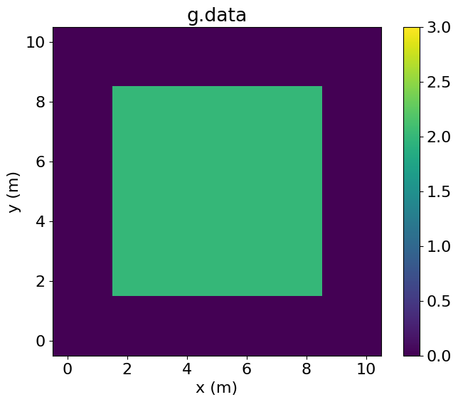

Note that we need not only iterate over the SubDomain on which our Function is defined. One can also iterate over any subset of this SubDomain. In this case, we define a new Left domain, alongside Intersection, which is the intersection of Left and Middle. We then define another Function h on left.

class Left(SubDomain):
    name = 'left'

    def define(self, dimensions):
        x, y = dimensions
        return {x: ('left', 6), y: y}


class Intersection(SubDomain):
    # Intersection of Left and Middle
    name = 'intersection'

    def define(self, dimensions):
        x, y = dimensions
        return {x: ('middle', 2, 5), y: ('middle', 2, 2)}


# Create the SubDomain instances
left = Left(grid=grid0)
intersection = Intersection(grid=grid0)

h = Function(name='h', grid=left)
h.data[:] = 1

Printing h.shape, we see that its size is also smaller than that of the Grid.

h.shape

(6, 11)

We can then define equations which act over the intersection of Middle and Left. These equations can operate on any of the Functions defined thus far.

#NBVAL_IGNORE_OUTPUT
# Equations operating on Functions defined on SubDomains must be applied over
# the SubDomain, or a SubDomain representing some subset thereof.

# Add h (defined on Left) to g (defined on Grid) over Intersection, and store result in g
eq_gh = Eq(g, g + h, subdomain=intersection)
# Add h (defined on Left) to f (defined on Middle) over Intersection, and store result in f
eq_fh = Eq(f, f + h, subdomain=intersection)

Operator([eq_gh, eq_fh])()

Operator `Kernel` ran in 0.01 s

PerformanceSummary([(PerfKey(name='section0', rank=None),
                     PerfEntry(time=0.000108, gflopss=0.0, gpointss=0.0, oi=0.0, ops=0, itershapes=[]))])

Plotting both g and f, we observe that both have been incremented by one (the value stored inh) over the intersection.

#NBVAL_IGNORE_OUTPUT
plt.imshow(g.data.T, vmin=0, vmax=3, origin='lower', extent=(-0.5, 10.5, -0.5, 10.5))
plt.colorbar()
plt.title("g.data")
plt.xlabel("x (m)")
plt.ylabel("y (m)")
plt.show()

plt.imshow(f.data.T, vmin=0, vmax=3, origin='lower', extent=(1.5, 8.5, 1.5, 8.5))
plt.colorbar()
plt.title("f.data")
plt.xlabel("x (m)")
plt.ylabel("y (m)")
plt.xlim(-0.5, 10.5)
plt.ylim(-0.5, 10.5)
plt.show()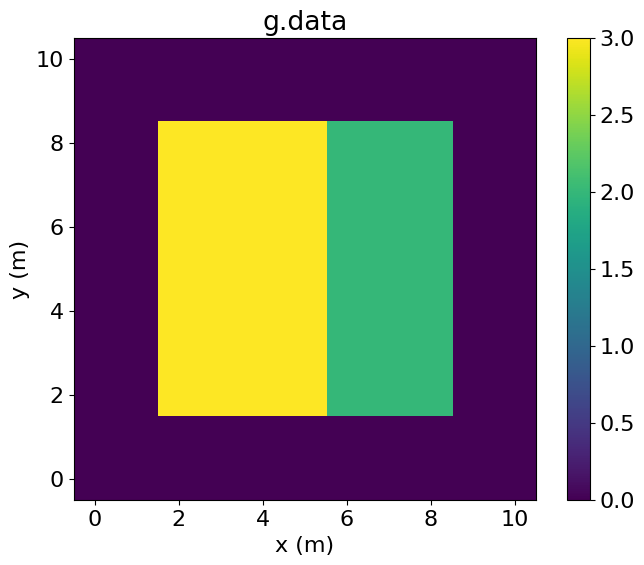

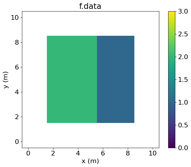
Finally, we can also take values from a Function defined on the Grid, operate on them, and store them in a Function defined on a SubDomain.

#NBVAL_IGNORE_OUTPUT
eq_gf = Eq(f, g)
Operator(eq_gf)()

Operator `Kernel` ran in 0.01 s

PerformanceSummary([(PerfKey(name='section0', rank=None),
                     PerfEntry(time=6.7e-05, gflopss=0.0, gpointss=0.0, oi=0.0, ops=0, itershapes=[]))])

Note that f now contains the same values as the central region of g.

#NBVAL_IGNORE_OUTPUT
plt.imshow(f.data.T, vmin=0, vmax=3, origin='lower', extent=(1.5, 8.5, 1.5, 8.5))
plt.colorbar()
plt.title("f.data")
plt.xlabel("x (m)")
plt.ylabel("y (m)")
plt.xlim(-0.5, 10.5)
plt.ylim(-0.5, 10.5)
plt.show()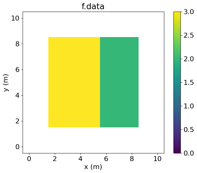

Sparse operations

Similarly, one can perform sparse operations such as injection into or interpolation off of Functions defined on SubDomains. This is performed as per the usual interface. Note however that the operation will be windowed to the SubDomain, not the Grid, even if it involves the interpolation of an expression featuring both Functions defined on a SubDomain and those defined on a Grid. This is because such an operation would be undefined outside a SubDomain.

We begin by constructing a SparseFunction.

src_rec = SparseFunction(name='srcrec', grid=grid0, npoint=1)
src_rec.coordinates.data[:] = np.array([[3., 3.]])

A simple interpolation operator is constructed as follows:

#NBVAL_IGNORE_OUTPUT
rec = src_rec.interpolate(expr=f)
Operator(rec)()

Operator `Kernel` ran in 0.01 s

PerformanceSummary([(PerfKey(name='section0', rank=None),
                     PerfEntry(time=9.999999999999999e-05, gflopss=0.0, gpointss=0.0, oi=0.0, ops=0, itershapes=[]))])

Printing srcrec.data, it is apparent that it now contains the value interpolated off of f.

src_rec.data

Data([3.], dtype=float32)

As aforementioned, one can also interpolate an expression featuring Functions defined on both the Grid and a SubDomain. This can be straightforwardly achieved as follows:

#NBVAL_IGNORE_OUTPUT
rec = src_rec.interpolate(expr=f+g)
Operator(rec)()

Operator `Kernel` ran in 0.01 s

PerformanceSummary([(PerfKey(name='section0', rank=None),
                     PerfEntry(time=7e-05, gflopss=0.0, gpointss=0.0, oi=0.0, ops=0, itershapes=[]))])

Note that since one of our previous operators set f equal to g over Middle, srcrec.data is now equal to 6.

src_rec.data

Data([6.], dtype=float32)

We can also inject into a Function defined on a SubDomain.

#NBVAL_IGNORE_OUTPUT
src = src_rec.inject(field=h, expr=1)
Operator(src)()

Operator `Kernel` ran in 0.01 s

PerformanceSummary([(PerfKey(name='section0', rank=None),
                     PerfEntry(time=8.599999999999999e-05, gflopss=0.0, gpointss=0.0, oi=0.0, ops=0, itershapes=[]))])

Plotting h.data, we see that a value of 1 has been injected. It is also apparent that this injection is aligned with the global grid.

#NBVAL_IGNORE_OUTPUT
plt.imshow(h.data.T, vmin=0, vmax=3, origin='lower', extent=(-0.5, 5.5, -0.5, 10.5))
plt.colorbar()
plt.title("h.data")
plt.xlabel("x (m)")
plt.ylabel("y (m)")
plt.xlim(-0.5, 10.5)
plt.ylim(-0.5, 10.5)
plt.show()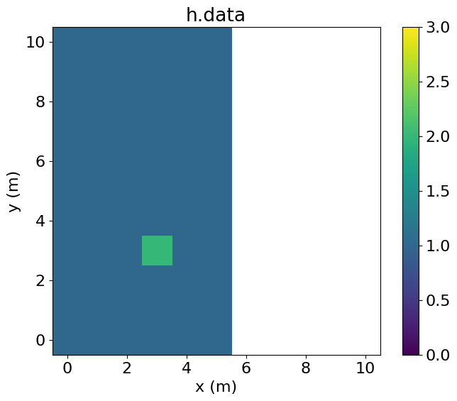

Snapshotting on a subset of a domain

We will now consider a practical application of this functionality. In many applications, it is necessary to capture snapshots of a simulation as it progresses. However, such snapshots may not be needed over the entirety of the domain. We can use a Function defined on the subset of the domain that we aim to capture to minimize the size of the arrays allocated.

In this case, we will consider the snapshotting of a seismic wavefield. In imaging workflows, there is no need to calculate an imaging condition in the water column, and thus no need to store snapshots of this portion of the domain.

We begin by setting up the grid parameters and velocity model.

origin = (0., 0.)
shape = (201, 201)
spacing = (5., 5.)
extent = tuple((sh-1)*sp for sh, sp in zip(shape, spacing))

# Layered model
vp = np.full(shape, 1.5)
for i in range(6):
    vp[:, 50+i*25:] += 0.3

We can then construct a Model. To highlight the use of Functions on SubDomains, we plot the padded velocity model, overlaying the interior domain (i.e. the core computational domain, excluding boundary layers) and the area of interest for snapshotting (excluding the water layer at the top).

#NBVAL_IGNORE_OUTPUT
model = Model(vp=vp, origin=origin, shape=shape, spacing=spacing,
              space_order=2, nbl=20, bcs="damp")

# Plot velocity model
plt.imshow(model.vp.data.T, extent=(-100, 1100., 1100., -100.))
plt.plot((0, 1000, 1000, 0, 0), (0, 0, 1000, 1000, 0), 'k', label="Main Domain")
plt.plot((0, 1000, 1000, 0, 0), (245, 245, 1000, 1000, 245), 'r--', label="Snapshotting Region")
plt.legend(loc='lower left')
plt.colorbar(label="km/s")
plt.xlabel("x (m)")
plt.ylabel("z (m)")
plt.show()

Operator `initdamp` ran in 0.01 s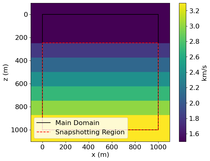

We then set up a SubDomain corresponding to this region.

class SnapshotDomain(SubDomain):
    name = 'snapshot'

    def define(self, dimensions):
        x, y = dimensions
        # Exclude damping layers and water column
        return {x: ('middle', 20, 20), y: ('middle', 70, 20)}


snapshotdomain = SnapshotDomain(grid=model.grid)

A trivial Operator can be used to check that the specified SubDomain is aligned as intended.

#NBVAL_IGNORE_OUTPUT
# Make a Function and set it equal to one to check the alignment of subdomain
test_func = Function(name='testfunc', grid=model.grid)
Operator(Eq(test_func, 1, subdomain=snapshotdomain))()

# Plotting the resultant field, we see that the incremented region aligns with our
# desired snapshotting region.
plt.imshow(test_func.data.T, extent=(-100, 1100., 1100., -100.))
plt.plot((0, 1000, 1000, 0, 0), (0, 0, 1000, 1000, 0), 'k', label="Main Domain")
plt.plot((0, 1000, 1000, 0, 0), (245, 245, 1000, 1000, 245), 'r--', label="Snapshotting Region")
plt.legend(loc='lower left')
plt.colorbar()
plt.xlabel("x (m)")
plt.ylabel("z (m)")
plt.show()

Operator `Kernel` ran in 0.01 s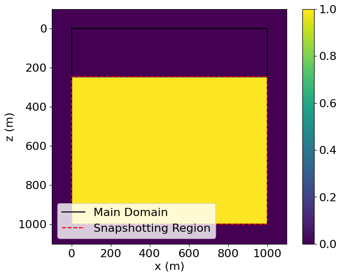

Now we set up a source.

# Set time range, source, source coordinates and receiver coordinates
t0 = 0.  # Simulation starts a t=0
tn = 500.  # Simulation lasts tn milliseconds
dt = 0.8*model.critical_dt  # Time step from model grid spacing
time_range = TimeAxis(start=t0, stop=tn, step=dt)
nt = time_range.num  # number of time steps

f0 = 0.040  # Source peak frequency is 10Hz (0.010 kHz)
src = RickerSource(name='src', grid=model.grid, f0=f0, time_range=time_range)  

src.coordinates.data[0, :] = np.array(model.domain_size) * .5
src.coordinates.data[0, -1] = 20.  # Depth is 20m

Snapshotting is specified as usual. The only difference is that grid=snapshotdomain is passed when instantiating the snapshot TimeFunction. For comparison, we also instantiate usavegrid in the conventional manner.

nsnaps = 30
factor = int(np.ceil(nt/nsnaps))

time_subsampled = ConditionalDimension('t_sub', parent=model.grid.time_dim, factor=factor)

u_save = TimeFunction(name='usave', grid=snapshotdomain, time_order=0, space_order=2,
                      save=nsnaps, time_dim=time_subsampled)

# "Normal" snapshotting for comparison
u_save_grid = TimeFunction(name='usavegrid', grid=model.grid, time_order=0, space_order=2,
                           save=nsnaps, time_dim=time_subsampled)

Comparing the size of usave, allocated on snapshotdomain, to usavegrid, allocated on model.grid, we see that the former has a substantially smaller underlying array than the latter. This yields notable memory savings.

memreduction = round(float(100*(u_save_grid.size - u_save.size)/u_save_grid.size), 2)

print(f"Using `Function`s on `SubDomain`s for this snapshot reduces memory requirements by {memreduction}%")

Using `Function`s on `SubDomain`s for this snapshot reduces memory requirements by 47.06%

We will solve the 2nd-order acoustic wave equation in this case. Note that both “normal” and subdomain snapshots are saved for comparison and plotting. In practice, one would only save the subdomain snapshots to minimise memory consumption.

#NBVAL_IGNORE_OUTPUT
u = TimeFunction(name="u", grid=model.grid, time_order=2, space_order=8)

pde = model.m * u.dt2 - u.laplace + model.damp * u.dt
stencil = Eq(u.forward, solve(pde, u.forward))
src_term = src.inject(field=u.forward, expr=src)

# Save both "normal" and subdomain snapshots for comparison
op = Operator([stencil] + [Eq(u_save, u, subdomain=snapshotdomain), Eq(u_save_grid, u)] + src_term)
op.apply(t_M=nt-2, dt=dt)

Operator `Kernel` ran in 0.09 s

PerformanceSummary([(PerfKey(name='section0', rank=None),
                     PerfEntry(time=0.0491209999999999, gflopss=0.0, gpointss=0.0, oi=0.0, ops=0, itershapes=[])),
                    (PerfKey(name='section1', rank=None),
                     PerfEntry(time=0.001683, gflopss=0.0, gpointss=0.0, oi=0.0, ops=0, itershapes=[])),
                    (PerfKey(name='section2', rank=None),
                     PerfEntry(time=0.002006, gflopss=0.0, gpointss=0.0, oi=0.0, ops=0, itershapes=[])),
                    (PerfKey(name='section3', rank=None),
                     PerfEntry(time=0.037044, gflopss=0.0, gpointss=0.0, oi=0.0, ops=0, itershapes=[]))])

We then visualise this process with an animation.

#NBVAL_SKIP
def animate_wavefield(f, fg, v, interval=100):
    """
    Create an animation of the wavefield.

    Parameters:
      f        : Snapshots on SubDomain
      fg       : Snapshots on Grid
      v        : Velocity model
      interval : Delay between frames in milliseconds (default: 100)
    """
    # Determine color limits based on full dataset (so they remain constant throughout)
    clip = 0.5
    vmax = clip * np.amax(np.abs(f.data))
    vmin = -vmax

    # Create the figure and axis
    fig, ax = plt.subplots()

    # Draw static elements
    # Velocity model (constant background)
    ax.imshow(v.data.T, cmap="Greys", extent=(-100, 1100, 1100, -100),
              alpha=0.4, zorder=3)
    # Snapshot region (red dashed line)
    ax.plot((0, 1000, 1000, 0, 0), (245, 245, 1000, 1000, 245),
            'r--', label="Snapshotting Region", zorder=4)

    # Draw time-dependent images
    # Initialize with the first frame (frame index 0)
    im_fg = ax.imshow(fg.data[0].T, vmin=vmin, vmax=vmax, cmap="Greys",
                      extent=(-100, 1100, 1100, -100), zorder=1)
    im_f  = ax.imshow(f.data[0].T, vmin=vmin, vmax=vmax, cmap='seismic',
                      extent=(0, 1000, 1000, 245), zorder=2)

    # Set axis limits
    ax.set_xlim(-100, 1100)
    ax.set_ylim(1100, -100)

    # Set axis labels
    ax.set_xlabel("x (m)")
    ax.set_ylabel("z (m)")

    def update(frame):
        """Update the images for frame 'frame'."""
        im_fg.set_data(fg.data[frame].T)
        im_f.set_data(f.data[frame].T)
        return im_fg, im_f

    # Determine the total number of frames from the first dimension of f.data
    n_frames = f.data.shape[0]

    # Create the animation
    ani = animation.FuncAnimation(fig, update, frames=n_frames, interval=interval, blit=True)
    plt.close()

    return ani

ani = animate_wavefield(u_save, u_save_grid, model.vp)

HTML(ani.to_html5_video())

assert np.isclose(np.linalg.norm(u_save.data), 54.026115, atol=0, rtol=1e-4)
assert np.isclose(np.linalg.norm(u_save_grid.data), 77.89853, atol=0, rtol=1e-4)

Acoustic-elastic coupling

Another application of the Functions on SubDomains functionality is for coupled physics problems in which certain fields are only required over a subset of the domain. By minimising the size of the allocated arrays, the memory required to run such complex models can be substantially reduced.

One such application is for efficiently handling propagation of seismic waves through both fluid and solid media. In the former, wave propagation is purely acoustic, whilst it is elastic in the latter. However, the elastic wave equation is substantially more expensive than its acoustic counterpart and features a greatly increased number of fields. Leveraging Functions defined on only a subset of the grid, such computations can be made substantially more memory-efficient.

In this particular case, we will have an upper acoustic domain and a lower elastic domain, overlapping in the center to enable coupling of the two simulations. The transition point will lie above the seafloor to simplify the coupling.

The two domains will be laid out as follows, with the overlap representing the transition zone.

#NBVAL_IGNORE_OUTPUT
plt.plot((-100., 1100., 1100., -100., -100.),
         (-100., -100., 520., 520., -100.),
         'k--', label='Acoustic')
plt.plot((-100., 1100., 1100., -100., -100.),
         (1100., 1100., 475., 475., 1100.),
         'r--', label='Elastic')

plt.legend(loc='lower left')
plt.xlabel("x (m)")
plt.ylabel("z (m)")
plt.xlim(-150, 1150)
plt.ylim(1150, -150)

plt.show()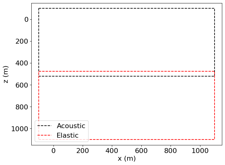

To achieve this setup, we will require a total of six SubDomains. These are as follows: * Two overlapping SubDomains, one for fields only required for acoustic propagation, and one for fields only required for elastic propagation * Two non-overlapping SubDomains, one for acoustic propagation, and one for elastic propagation * Two SubDomains to act as ‘halos’ for coupling the acoustic and elastic models in the upper and lower halves of the transition zone.

so = 8  # Space order
grid1 = Grid(shape=(241, 241), extent=(1200., 1200.), origin=(-100., -100.))


# Acoustic-elastic transition at index 120 (this index is the first elastic one)
class Upper(SubDomain):
    """Upper iteration subdomain"""
    name = 'upper'

    def define(self, dimensions):
        x, y = dimensions
        # Note: uses middle to allow MPI distribution. If MPI is not needed or anticipated
        # then one could use left/right instead
        return {x: x, y: ('middle', 0, 121)}  # 121 + so//2


class Lower(SubDomain):
    """Lower iteration subdomain"""
    name = 'lower'

    def define(self, dimensions):
        x, y = dimensions
        return {x: x, y: ('middle', 120, 0)}  # 120 + so//2


class UpperTransition(SubDomain):
    """Upper transition zone"""
    name = 'uppertransition'

    def define(self, dimensions):
        x, y = dimensions
        return {x: x, y: ('middle', 116, 121)}  # 116 + 121 = 241 - so//2


class LowerTransition(SubDomain):
    """Lower transition zone"""
    name = 'lowertransition'

    def define(self, dimensions):
        x, y = dimensions
        return {x: x, y: ('middle', 120, 117)}  # 120 + 117 = 241 - so//2


class UpperField(SubDomain):
    """Upper subdomain to define fields over"""
    name = 'upperfields'

    def define(self, dimensions):
        x, y = dimensions
        return {x: x, y: ('middle', 0, 117)}  # 121 - so//2


class LowerField(SubDomain):
    """Lower subdomain to define fields over"""
    name = 'lowerfields'

    def define(self, dimensions):
        x, y = dimensions
        return {x: x, y: ('middle', 116, 0)}  # 120 - so//2


# Iteration domains
upper = Upper(grid=grid1)
lower = Lower(grid=grid1)
uppertransition = UpperTransition(grid=grid1)
lowertransition = LowerTransition(grid=grid1)

# Field domains
upperfield = UpperField(grid=grid1)
lowerfield = LowerField(grid=grid1)

As before, it is often helpful to create a trivial Operator to check the alignment and layout of the SubDomains created, particularly when a large number are present. Doing so also illustrates how the transition zone is split into upper and lower regions, acting as halos for the elastic and acoustic models respectively.

#NBVAL_IGNORE_OUTPUT
# Make a trivial operator to check location of fields
test_func = Function(name='testfunc', grid=grid1)
Operator([Eq(test_func, 1, subdomain=upper),
          Eq(test_func, 1, subdomain=lower),
          Eq(test_func, test_func + 1, subdomain=uppertransition),
          Eq(test_func, test_func + 2, subdomain=lowertransition)])()

plt.imshow(test_func.data.T, extent=(-100., 1100., 1100., -100.))
plt.colorbar()
plt.xlabel("x (m)")
plt.ylabel("z (m)")
plt.show()

Operator `Kernel` ran in 0.01 s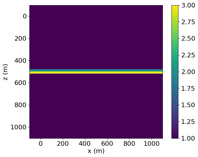

We now define the necessary fields. Only the damping and P-wave velocity fields are required throughout the domain. Thus all remaining fields are defined on either upperfield or lowerfield, these being the overlapped SubDomains.

# Define the fields
# Fields present everywhere
damp = Function(name='damp', grid=grid1, space_order=so)
cp = Function(name='cp', grid=grid1, space_order=so)

# Fields only present in the upper domain
p = TimeFunction(name='p', grid=upperfield, space_order=so, time_order=2)

# Fields only present in the lower domain
cs = Function(name='cs', grid=lowerfield, space_order=so)
ro = Function(name='ro', grid=lowerfield, space_order=so)
tau = TensorTimeFunction(name='tau', grid=lowerfield, space_order=so)
v = VectorTimeFunction(name='v', grid=lowerfield, space_order=so)

# Intialise parameter fields
ro.data[:] = 1
cp.data[:] = 1.5

# Add an elastic layer below the acoustic-elastic transition
cp.data[:, -100:] = 2.5
cs.data[:, -100:] = 1.5
cp.data[:, -75:] = 3.0
cs.data[:, -75:] = 2.0
cp.data[:, -50:] = 3.5
cs.data[:, -50:] = 2.5
cp.data[:, -25:] = 4.
cs.data[:, -25:] = 3.

# Fill the damping field
maxtaper = 0.5
taper = maxtaper*(0.5 - 0.5*np.cos(np.linspace(0., np.pi, 20)))
damp.data[-20:] += taper[:, np.newaxis]
damp.data[:20] += taper[::-1, np.newaxis]
damp.data[:, -20:] += taper[:]
damp.data[:, :20] += taper[::-1]

Source terms are defined as per usual.

# Set time range, source, source coordinates and receiver coordinates
t0 = 0.  # Simulation starts a t=0
tn = 400.  # Simulation lasts tn milliseconds
dt = float(0.1*np.amin(grid1.spacing)/np.amax(cp.data))  # Time step from grid spacing
time_range = TimeAxis(start=t0, stop=tn, step=dt)
nt = time_range.num  # number of time steps

f0 = 0.030  # Source peak frequency is 30Hz (0.030 kHz)
src = RickerSource(name='src', grid=grid1, f0=f0, time_range=time_range)  

src.coordinates.data[0, :] = 500.
src.coordinates.data[0, -1] = 350.  # Depth is 350m

Receivers will be placed on the seafloor. Note that this is below the transition, in the elastic zone.

rec = Receiver(name='rec', grid=grid1, npoint=101, time_range=time_range)

rec.coordinates.data[:, 0] = np.linspace(0., 1000., 101)
rec.coordinates.data[:, 1] = 600.

Define some material parameters.

b = 1/ro
mu = cs**2*ro
lam = cp**2*ro - 2*mu

Update and coupling equations are specified. Note that it is important to specify a SubDomain when an expression contains Functions defined on SubDomains.

# Acoustic update
pde_p = p.dt2 - cp**2*p.laplace + damp*p.dt
eq_p = Eq(p.forward, solve(pde_p, p.forward), subdomain=upper)

# Elastic update
pde_v = v.dt - b*div(tau) + damp*v.forward
pde_tau = tau.dt - lam*diag(div(v.forward)) - mu*(grad(v.forward) + grad(v.forward).transpose(inner=False)) + damp*tau.forward

eq_v = Eq(v.forward, solve(pde_v, v.forward), subdomain=lowerfield)
eq_t = Eq(tau.forward, solve(pde_tau, tau.forward), subdomain=lower)

# Coupling: p -> txx, tyy
eq_txx_tr = Eq(tau[0, 0].forward, p.forward, subdomain=uppertransition)
eq_tyy_tr = Eq(tau[1, 1].forward, p.forward, subdomain=uppertransition)
# Coupling: txx, tyy -> p
eq_p_tr = Eq(p.forward, (tau[0, 0].forward + tau[1, 1].forward)/2, subdomain=lowertransition)

Source and receiver terms are defined.

src_term = src.inject(field=p.forward, expr=src)
rec_term = rec.interpolate(expr=tau[0, 0].forward+tau[1, 1].forward)

Now build and run the Operator.

#NBVAL_IGNORE_OUTPUT
from devito import switchconfig

# Note: switchconfig(safe_math=True) is only required here to get consistent norms for testing purposes
# This is not required more widely and can be omitted in practical applications
with switchconfig(safe_math=True):
    op1 = Operator([eq_v,
                eq_p, eq_t,
                eq_p_tr, eq_txx_tr, eq_tyy_tr]
               + src_term + rec_term)
    op1(dt=dt)

Operator `Kernel` ran in 0.74 s

Overlaying the wavefields, we see that they are correctly coupled and aligned.

#NBVAL_IGNORE_OUTPUT
vmax_p = np.amax(np.abs(p.data[-1]))
vmax_tau = np.amax(np.abs((tau[0, 0].data[-1] + tau[1, 1].data[-1])/2))
vmax = max(vmax_p, vmax_tau)

plt.imshow(cp.data.T, cmap='Greys', extent=(-100, 1100, 1100, -100))
plt.imshow(p.data[-1].T,
           vmax=vmax, vmin=-vmax, cmap='Greys',
           extent=(-100, 1100, 520, -100),
           alpha=0.6)
plt.imshow((tau[0, 0].data[-1].T + tau[1, 1].data[-1].T)/2,
           vmax=vmax, vmin=-vmax, cmap='seismic',
           extent=(-100, 1100, 1100, 475), alpha=0.6)

plt.plot((-100., 1100., 1100., -100., -100.),
         (-100., -100., 520., 520., -100.),
         'k--', label='Acoustic')
plt.plot((-100., 1100., 1100., -100., -100.),
         (1100., 1100., 475., 475., 1100.),
         'r--', label='Elastic')

plt.legend()


plt.xlim(-100, 1100)
plt.ylim(1100, -100)
plt.xlabel("x (m)")
plt.ylabel("z (m)")
plt.show()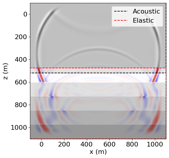

We can also view the shot record recorded at the ocean-bottom receivers.

#NBVAL_IGNORE_OUTPUT
vmax = 0.05*np.amax(np.abs(rec.data))
plt.imshow(rec.data, cmap='Greys', aspect='auto', vmax=vmax, vmin=-vmax)
plt.xlabel("Receiver number")
plt.ylabel("Sample")
plt.show()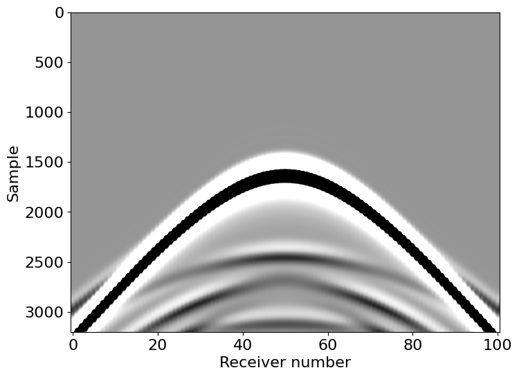

assert np.isclose(np.linalg.norm(rec.data), 4263.511, atol=0, rtol=1e-4)