from examples.cfd import plot_field, init_hat
import numpy as np
%matplotlib inline

# Some variable declarations
nx = 100
ny = 100
nt = 1000

nu = 0.15  # the value of base viscosity

offset = 1  # Used for field definition

visc = np.full((nx, ny), nu)  # Initialize viscosity
visc[nx//4-offset:nx//4+offset, 1:-1] = 0.0001  # Adding a material with different viscosity
visc[1:-1, nx//4-offset:nx//4+offset] = 0.0001
visc[3*nx//4-offset:3*nx//4+offset, 1:-1] = 0.0001

visc_nb = visc[1:-1, 1:-1]

dx = 2. / (nx - 1)
dy = 2. / (ny - 1)
sigma = .25
dt = sigma * dx * dy / nu


# Initialize our field

# Initialise u with hat function
u_init = np.empty((nx, ny))
init_hat(field=u_init, dx=dx, dy=dy, value=1)
u_init[10:-10, 10:-10] = 1.5


zmax = 2.5 # zmax for plottingExample 3 , part B: Diffusion for non uniform material properties
In this example we will look at the diffusion equation for non uniform material properties and how to handle second-order derivatives. For this, we will reuse Devito’s .laplace short-hand expression outlined in the previous example and demonstrate it using the examples from step 7 of the original tutorial. This example is an enhancement of 03_diffusion in terms of having non-uniform viscosity as opposed to the constant \(\nu\). This example introduces the use of Function in order to create this non-uniform space.
So, the equation we are now trying to implement is
\[\frac{\partial u}{\partial t} = \nu(x,y) \frac{\partial ^2 u}{\partial x^2} + \nu(x,y) \frac{\partial ^2 u}{\partial y^2}\]
In our case \(\nu\) is not uniform and \(\nu(x,y)\) represents spatially variable viscosity. To discretize this equation we will use central differences and reorganizing the terms yields
\[\begin{align} u_{i,j}^{n+1} = u_{i,j}^n &+ \frac{\nu(x,y) \Delta t}{\Delta x^2}(u_{i+1,j}^n - 2 u_{i,j}^n + u_{i-1,j}^n) \\ &+ \frac{\nu(x,y) \Delta t}{\Delta y^2}(u_{i,j+1}^n-2 u_{i,j}^n + u_{i,j-1}^n) \end{align}\]
As usual, we establish our baseline experiment by re-creating some of the original example runs. So let’s start by defining some parameters.
We now set up the diffusion operator as a separate function, so that we can re-use if for several runs.
def diffuse(u, nt, visc):
    for _ in range(nt + 1):
        un = u.copy()
        u[1:-1, 1:-1] = (un[1:-1, 1:-1] +
                        visc*dt / dy**2 * (un[1:-1, 2:] - 2 * un[1:-1, 1:-1] + un[1:-1, 0:-2]) +
                        visc*dt / dx**2 * (un[2:, 1: -1] - 2 * un[1:-1, 1:-1] + un[0:-2, 1:-1]))
        u[0, :] = 1
        u[-1, :] = 1
        u[:, 0] = 1
        u[:, -1] = 1
Now let’s take this for a spin. In the next two cells we run the same diffusion operator for a varying number of timesteps to see our “hat function” dissipate to varying degrees.
# NBVAL_IGNORE_OUTPUT
# Plot material according to viscosity, uncomment to plot
import matplotlib.pyplot as plt
plt.imshow(visc_nb, cmap='Greys', interpolation='nearest')
# Field initialization
u = u_init
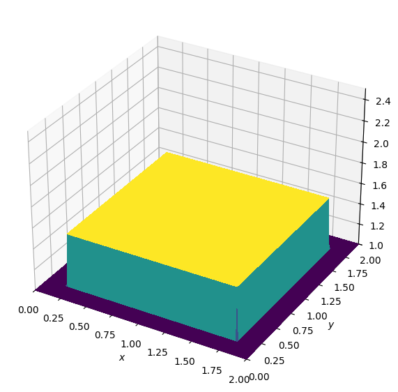
print("Initial state")
plot_field(u, zmax=zmax)
diffuse(u, nt, visc_nb)
print("After", nt, "timesteps")
plot_field(u, zmax=zmax)
diffuse(u, nt, visc_nb)
print("After another", nt, "timesteps")
plot_field(u, zmax=zmax)Initial state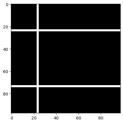
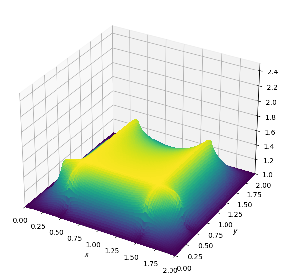
After 1000 timesteps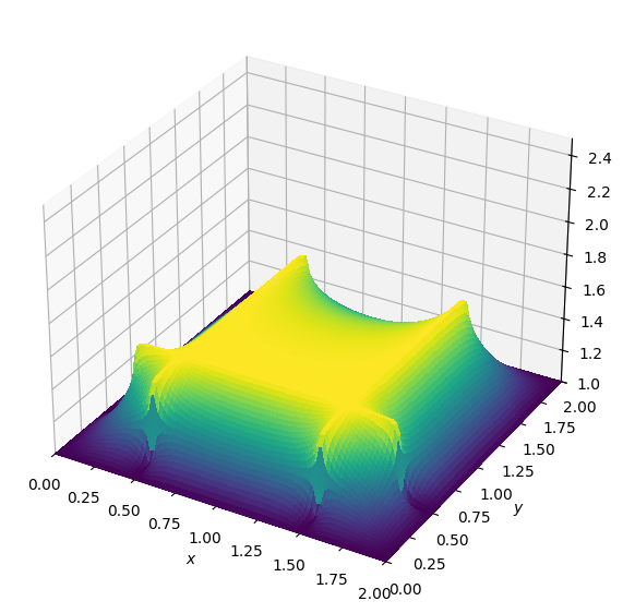
After another 1000 timesteps
You can notice that the area with lower viscosity is not diffusing its heat as quickly as the area with higher viscosity.
# NBVAL_IGNORE_OUTPUT

# Field initialization
u = u_init


diffuse(u, nt, visc_nb)
print("After", nt, "timesteps")
plot_field(u, zmax=zmax)
After 1000 timesteps
Excellent. Now for the Devito part, we need to note one important detail to our previous examples: we now have a second-order derivative. So, when creating our TimeFunction object we need to tell it about our spatial discretization by setting space_order=2. We also use the notation u.laplace outlined previously to denote all second order derivatives in space, allowing us to reuse this code for 2D and 3D examples.
from devito import Grid, TimeFunction, Eq, solve, Function

# Initialize `u` for space order 2
grid = Grid(shape=(nx, ny), extent=(2., 2.))

# Create an operator with second-order derivatives
a = Function(name='a', grid=grid)  # Define as Function
a.data[:] = visc  # Pass the viscosity in order to be used in the operator.


u = TimeFunction(name='u', grid=grid, space_order=2)

# Create an equation with second-order derivatives
eq = Eq(u.dt, a * u.laplace)
stencil = solve(eq, u.forward)
eq_stencil = Eq(u.forward, stencil)

eq_stencil
\(\displaystyle u(t + dt, x, y) = dt \left(\left(\frac{\partial^{2}}{\partial x^{2}} u(t, x, y) + \frac{\partial^{2}}{\partial y^{2}} u(t, x, y)\right) a(x, y) + \frac{u(t, x, y)}{dt}\right)\)
Great. Now all that is left is to put it all together to build the operator and use it on our examples. For illustration purposes we will do this in one cell, including update equation and boundary conditions.
# NBVAL_IGNORE_OUTPUT
from devito import Operator, Eq, solve, Function


# Reset our data field and ICs
init_hat(field=u.data[0], dx=dx, dy=dy, value=1.)

# Field initialization
u.data[0] = u_init


# Create an operator with second-order derivatives
a = Function(name='a', grid=grid)
a.data[:] = visc

eq = Eq(u.dt, a * u.laplace, subdomain=grid.interior)
stencil = solve(eq, u.forward)
eq_stencil = Eq(u.forward, stencil)

# Create boundary condition expressions
x, y = grid.dimensions
t = grid.stepping_dim
bc = [Eq(u[t+1, 0, y], 1.)]  # left
bc += [Eq(u[t+1, nx-1, y], 1.)]  # right
bc += [Eq(u[t+1, x, ny-1], 1.)]  # top
bc += [Eq(u[t+1, x, 0], 1.)]  # bottom


op = Operator([eq_stencil] + bc)
op(time=nt, dt=dt, a=a)

print("After", nt, "timesteps")
plot_field(u.data[0], zmax=zmax)

op(time=nt, dt=dt, a=a)
print("After another", nt, "timesteps")
plot_field(u.data[0], zmax=zmax)
Operator `Kernel` ran in 0.03 sAfter 1000 timesteps
Operator `Kernel` ran in 0.03 sAfter another 1000 timesteps