from devito import *The Devito domain specific language: an overview
This notebook presents an overview of the Devito symbolic language, used to express and discretise operators, in particular partial differential equations (PDEs).
For convenience, we import all Devito modules:
From equations to code in a few lines of Python
The main objective of this tutorial is to demonstrate how Devito and its SymPy-powered symbolic API can be used to solve partial differential equations using the finite difference method with highly optimized stencils in a few lines of Python. We demonstrate how computational stencils can be derived directly from the equation in an automated fashion and how Devito can be used to generate and execute, at runtime, the desired numerical scheme in the form of optimized C code.
Defining the physical domain
Before we can begin creating finite-difference (FD) stencils we will need to give Devito a few details regarding the computational domain within which we wish to solve our problem. For this purpose we create a Grid object that stores the physical extent (the size) of our domain and knows how many points we want to use in each dimension to discretise our data.
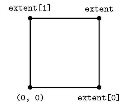
grid = Grid(shape=(5, 6), extent=(1., 1.))
grid
Grid[extent=(1.0, 1.0), shape=(5, 6), dimensions=(x, y)]Functions and data
To express our equation in symbolic form and discretise it using finite differences, Devito provides a set of Function types. A Function object:
- Behaves like a
sympy.Functionsymbol - Manages data associated with the symbol
To get more information on how to create and use a Function object, or any type provided by Devito, we can take a look at the documentation.
print(Function.__doc__)
    Tensor symbol representing a discrete function in symbolic equations.

    A Function carries multi-dimensional data and provides operations to create
    finite-differences approximations.

    A Function encapsulates space-varying data; for data that also varies in time,
    use TimeFunction instead.

    Parameters
    ----------
    name : str
        Name of the symbol.
    grid : Grid, optional
        Carries shape, dimensions, and dtype of the Function. When grid is not
        provided, shape and dimensions must be given. For MPI execution, a
        Grid is compulsory.
    space_order : int or 3-tuple of ints, optional, default=1
        Discretisation order for space derivatives.
        `space_order` also impacts the number of points available around a
        generic point of interest.  By default, `space_order` points are
        available on both sides of a generic point of interest, including those
        nearby the grid boundary. Sometimes, fewer points suffice; in other
        scenarios, more points are necessary. In such cases, instead of an
        integer, one can pass:
          * a 3-tuple `(o, lp, rp)` indicating the discretization order
            (`o`) as well as the number of points on the left (`lp`) and
            right (`rp`) sides of a generic point of interest;
          * a 2-tuple `(o, ((lp0, rp0), (lp1, rp1), ...))` indicating the
            discretization order (`o`) as well as the number of points on
            the left/right sides of a generic point of interest for each
            SpaceDimension.
    interp_order: int, optional, default=2
        Order of the interpolation scheme used to evaluate the Function at
        non-grid points (e.g., when using a Function as a parameter to be
        evaluated at a staggered location).
    shape : tuple of ints, optional
        Shape of the domain region in grid points. Only necessary if `grid`
        isn't given.
    dimensions : tuple of Dimension, optional
        Dimensions associated with the object. Only necessary if `grid` isn't
        given.
    dtype : data-type, optional, default=np.float32
        Any object that can be interpreted as a numpy data type.
    staggered : Dimension or tuple of Dimension or Stagger, optional, default=None
        Define how the Function is staggered.
    initializer : callable or any object exposing the buffer interface, default=None
        Data initializer. If a callable is provided, data is allocated lazily.
    allocator : MemoryAllocator, optional
        Controller for memory allocation. To be used, for example, when one wants
        to take advantage of the memory hierarchy in a NUMA architecture. Refer to
        `default_allocator.__doc__` for more information.

    Examples
    --------
    Creation

    >>> from devito import Grid, Function
    >>> grid = Grid(shape=(4, 4))
    >>> f = Function(name='f', grid=grid)
    >>> f
    f(x, y)
    >>> g = Function(name='g', grid=grid, space_order=2)
    >>> g
    g(x, y)

    First-order derivatives through centered finite-difference approximations

    >>> f.dx
    Derivative(f(x, y), x)
    >>> f.dy
    Derivative(f(x, y), y)
    >>> g.dx
    Derivative(g(x, y), x)
    >>> (f + g).dx
    Derivative(f(x, y) + g(x, y), x)

    First-order derivatives through left/right finite-difference approximations

    >>> f.dxl
    Derivative(f(x, y), x)

    Note that the fact that it's a left-derivative isn't captured in the representation.
    However, upon derivative expansion, this becomes clear

    >>> f.dxl.evaluate
    f(x, y)/h_x - f(x - h_x, y)/h_x
    >>> f.dxr
    Derivative(f(x, y), x)

    Second-order derivative through centered finite-difference approximation

    >>> g.dx2
    Derivative(g(x, y), (x, 2))

    Notes
    -----
    The parameters must always be given as keyword arguments, since SymPy
    uses `*args` to (re-)create the dimension arguments of the symbolic object.
Ok, let’s create a function \(f(x, y)\) and look at the data Devito has associated with it. Please note that it is important to use explicit keywords, such as name or grid when creating Function objects.
f = Function(name='f', grid=grid)
f
\(\displaystyle f(x, y)\)
f.dataData([[0., 0., 0., 0., 0., 0.],
[0., 0., 0., 0., 0., 0.],
[0., 0., 0., 0., 0., 0.],
[0., 0., 0., 0., 0., 0.],
[0., 0., 0., 0., 0., 0.]], dtype=float32)By default, Devito Function objects use the spatial dimensions (x, y) for 2D grids and (x, y, z) for 3D grids. To solve a PDE over several timesteps a time dimension is also required by our symbolic function. For this Devito provides an additional function type, the TimeFunction, which incorporates the correct dimension along with some other intricacies needed to create a time stepping scheme.
g = TimeFunction(name='g', grid=grid)
g
\(\displaystyle g(t, x, y)\)
Since the default time order of a TimeFunction is 1, the shape of f is (2, 5, 6), i.e. Devito has allocated two buffers to represent g(t, x, y) and g(t + dt, x, y):
g.shape(2, 5, 6)Derivatives of symbolic functions
The functions we have created so far all act as sympy.Function objects, which means that we can form symbolic derivative expressions from them. Devito provides a set of shorthand expressions (implemented as Python properties) that allow us to generate finite differences in symbolic form. For example, the property f.dx denotes \(\frac{\partial}{\partial x} f(x, y)\) - only that Devito has already discretised it with a finite difference expression. There are also a set of shorthand expressions for left (backward) and right (forward) derivatives:
| Derivative | Shorthand | Discretised | Stencil |
|---|---|---|---|
| \(\frac{\partial}{\partial x}f(x, y)\) (right) | f.dxr |
\(\frac{f(x+h_x,y)}{h_x} - \frac{f(x,y)}{h_x}\) | 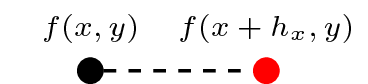 |
| \(\frac{\partial}{\partial x}f(x, y)\) (left) | f.dxl |
\(\frac{f(x,y)}{h_x} - \frac{f(x-h_x,y)}{h_x}\) | 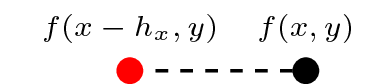 |
A similar set of expressions exist for each spatial dimension defined on our grid, for example f.dy and f.dyl. Obviously, one can also take derivatives in time of TimeFunction objects. For example, to take the first derivative in time of g you can simply write:
g.dt\(\displaystyle \frac{\partial}{\partial t} g(t, x, y)\)
We may also want to take a look at the stencil Devito will generate based on the chosen discretisation:
g.dt.evaluate\(\displaystyle - \frac{g(t, x, y)}{dt} + \frac{g(t + dt, x, y)}{dt}\)
There also exist convenient shortcuts to express the forward and backward stencil points, g(t+dt, x, y) and g(t-dt, x, y).
g.forward\(\displaystyle g(t + dt, x, y)\)
g.backward\(\displaystyle g(t - dt, x, y)\)
And of course, there’s nothing to stop us taking derivatives on these objects:
g.forward.dt\(\displaystyle \frac{\partial}{\partial t} g(t + dt, x, y)\)
g.forward.dy\(\displaystyle \frac{\partial}{\partial y} g(t + dt, x, y)\)
45-Degree Rotated Finite Differences
Rotated finite differences, when applied at a 45-degree angle, harness a unique isotropic discretization strategy for solving partial differential equations (PDEs) on a two-dimensional grid. This approach modifies the traditional finite difference stencil by rotating the coordinate system, specifically by 45 degrees, to better align with the problem’s directional sensitivities. The mathematical transformations for this rotation are straightforward yet powerful, given by:
\[x' = \frac{x + y}{\sqrt{2}}, \quad y' = \frac{y - x}{\sqrt{2}}\]
where \((x, y)\) and \((x', y')\) are the original and rotated coordinates, respectively.
Mathematical Definitions
The partial derivatives in the rotated system become:
\[\frac{\partial f}{\partial x'} \approx \frac{f(x'+\Delta x', y') - f(x'-\Delta x', y')}{2\Delta x'}\] \[\frac{\partial f}{\partial y'} \approx \frac{f(x', y'+\Delta y') - f(x', y'-\Delta y')}{2\Delta y'}\]
Here, \(\Delta x'\) and \(\Delta y'\) represent the grid spacing in the rotated coordinates, which effectively equals the original grid spacing scaled by \(\sqrt{2}\).
Use Case and Advantages
The 45-degree rotated finite difference method shines in scenarios where PDEs exhibit significant diagonal features or anisotropic behaviors. Traditional finite difference stencils, aligned with the Cartesian grid, can introduce numerical errors or fail to capture the essence of such phenomena accurately. By rotating the stencil, this method ensures a more symmetric and isotropic treatment of the grid points, leading to enhanced accuracy and stability in numerical simulations.
Advantages Include:
- Reduced Numerical Dispersion: By capturing diagonal relationships more naturally, this method mitigates the dispersion errors commonly seen in conventional finite difference schemes.
- Enhanced Anisotropy Representation: It offers a superior framework for simulating physical phenomena where directional dependencies are not aligned with the standard Cartesian axes.
- Improved Accuracy: The isotropic discretization helps in achieving higher accuracy, especially for problems with inherent diagonal or anisotropic features.
The 45-degree rotated finite difference method is a powerful tool for numerical analysts and engineers, providing a nuanced approach to solving complex PDEs with improved fidelity to the physical and geometric intricacies of the underlying problem.
f.dx45\(\displaystyle \frac{\partial}{\partial x} f(x, y)\)
f.dx45.evaluate\(\displaystyle \left(- \frac{f(x, y)}{2 h_{x}} + \frac{f(x + h_x, y - h_y)}{2 h_{x}}\right) + \left(- \frac{f(x, y)}{2 h_{x}} + \frac{f(x + h_x, y + h_y)}{2 h_{x}}\right)\)
A linear convection operator
Note: The following example is derived from step 5 in the excellent tutorial series CFD Python: 12 steps to Navier-Stokes.
In this simple example we will show how to derive a very simple convection operator from a high-level description of the governing equation. We will go through the process of deriving a discretised finite difference formulation of the state update for the field variable \(u\), before creating a callable Operator object. Luckily, the automation provided by SymPy makes the derivation very nice and easy.
The governing equation we want to implement is the linear convection equation: \[\frac{\partial u}{\partial t}+c\frac{\partial u}{\partial x} + c\frac{\partial u}{\partial y} = 0.\]
Before we begin, we must define some parameters including the grid, the number of timesteps and the timestep size. We will also initialize our velocity u with a smooth field:
from examples.cfd import init_smooth, plot_field

nt = 100  # Number of timesteps
dt = 0.2 * 2. / 80  # Timestep size (sigma=0.2)
c = 1  # Value for c

# Then we create a grid and our function
grid = Grid(shape=(81, 81), extent=(2., 2.))
u = TimeFunction(name='u', grid=grid)

# We can now set the initial condition and plot it
init_smooth(field=u.data[0], dx=grid.spacing[0], dy=grid.spacing[1])
init_smooth(field=u.data[1], dx=grid.spacing[0], dy=grid.spacing[1])

plot_field(u.data[0])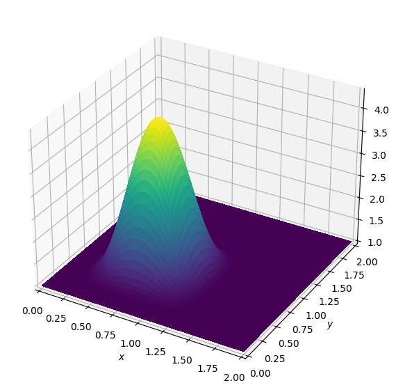
Next, we wish to discretise our governing equation so that a functional Operator can be created from it. We begin by simply writing out the equation as a symbolic expression, while using shorthand expressions for the derivatives provided by the Function object. This will create a symbolic object of the dicretised equation.
Using the Devito shorthand notation, we can express the governing equations as:
eq = Eq(u.dt + c * u.dxl + c * u.dyl)
eq
\(\displaystyle \frac{\partial}{\partial x} u(t, x, y) + \frac{\partial}{\partial y} u(t, x, y) + \frac{\partial}{\partial t} u(t, x, y) = 0\)
We now need to rearrange our equation so that the term \(u(t+dt, x, y)\) is on the left-hand side, since it represents the next point in time for our state variable \(u\). Devito provides a utility called solve, built on top of SymPy’s solve, to rearrange our equation so that it represents a valid state update for \(u\). Here, we use solve to create a valid stencil for our update to u(t+dt, x, y):
stencil = solve(eq, u.forward)
update = Eq(u.forward, stencil)
update
\(\displaystyle u(t + dt, x, y) = dt \left(- \frac{\partial}{\partial x} u(t, x, y) - \frac{\partial}{\partial y} u(t, x, y) + \frac{u(t, x, y)}{dt}\right)\)
The right-hand side of the ‘update’ equation should be a stencil of the shape 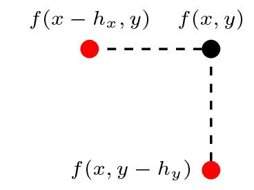
Once we have created this ‘update’ expression, we can create a Devito Operator. This Operator will basically behave like a Python function that we can call to apply the created stencil over our associated data, as long as we provide all necessary unknowns. In this case we need to provide the number of timesteps to compute via the keyword time and the timestep size via dt (both have been defined above):
op = Operator(update, opt='noop')
op(time=nt+1, dt=dt)

plot_field(u.data[0])
Operator `Kernel` ran in 0.06 s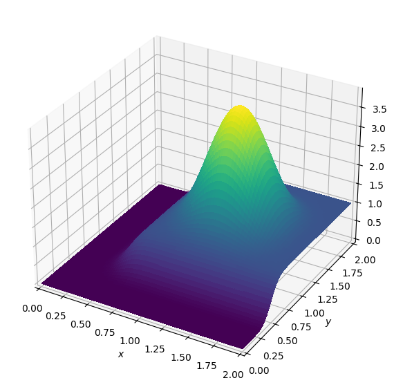
Note that the real power of Devito is hidden within Operator, it will automatically generate and compile the optimized C code. We can look at this code (noting that this is not a requirement of executing it) via:
print(op.ccode)/* Devito generated code for Operator `Kernel` */
#define _POSIX_C_SOURCE 200809L
#define START(S) struct timeval start_ ## S , end_ ## S ; gettimeofday(&start_ ## S , NULL);
#define STOP(S,T) gettimeofday(&end_ ## S, NULL); T->S += (double)(end_ ## S .tv_sec-start_ ## S.tv_sec)+(double)(end_ ## S .tv_usec-start_ ## S .tv_usec)/1000000;
#include "stdlib.h"
#include "math.h"
#include "sys/time.h"
#include "omp.h"
struct dataobj
{
void *restrict data;
int * size;
unsigned long nbytes;
unsigned long * npsize;
unsigned long * dsize;
int * hsize;
int * hofs;
int * oofs;
void * dmap;
} ;
struct profiler
{
double section0;
} ;
int Kernel(struct dataobj *restrict u_vec, const float dt, const float h_x, const float h_y, const int time_M, const int time_m, const int x_M, const int x_m, const int y_M, const int y_m, const int nthreads, struct profiler * timers)
{
float (*restrict u)[u_vec->size[1]][u_vec->size[2]] __attribute__ ((aligned (64))) = (float (*)[u_vec->size[1]][u_vec->size[2]]) u_vec->data;
for (int time = time_m, t0 = (time)%(2), t1 = (time + 1)%(2); time <= time_M; time += 1, t0 = (time)%(2), t1 = (time + 1)%(2))
{
START(section0)
#pragma omp parallel num_threads(nthreads)
{
#pragma omp for collapse(2) schedule(dynamic,1)
for (int x = x_m; x <= x_M; x += 1)
{
for (int y = y_m; y <= y_M; y += 1)
{
u[t1][x + 1][y + 1] = dt*(-(-u[t0][x][y + 1]/h_x + u[t0][x + 1][y + 1]/h_x) - (-u[t0][x + 1][y]/h_y + u[t0][x + 1][y + 1]/h_y) + u[t0][x + 1][y + 1]/dt);
}
}
}
STOP(section0,timers)
}
return 0;
}
Second derivatives and high-order stencils
In the above example only a combination of first derivatives was present in the governing equation. However, second (or higher) order derivatives are often present in scientific problems of interest, notably any PDE modeling diffusion. To generate second order derivatives we must give the devito.Function object another piece of information: the desired discretisation of the stencil(s).
First, lets define a simple second derivative in x, for which we need to give \(u\) a space_order of (at least) 2. The shorthand for this second derivative is u.dx2.
u = TimeFunction(name='u', grid=grid, space_order=2)
u.dx2
\(\displaystyle \frac{\partial^{2}}{\partial x^{2}} u(t, x, y)\)
u.dx2.evaluate\(\displaystyle - \frac{2.0 u(t, x, y)}{h_{x}^{2}} + \frac{u(t, x - h_x, y)}{h_{x}^{2}} + \frac{u(t, x + h_x, y)}{h_{x}^{2}}\)
We can increase the discretisation arbitrarily if we wish to specify higher order FD stencils:
u = TimeFunction(name='u', grid=grid, space_order=4)
u.dx2
\(\displaystyle \frac{\partial^{2}}{\partial x^{2}} u(t, x, y)\)
u.dx2.evaluate\(\displaystyle - \frac{2.5 u(t, x, y)}{h_{x}^{2}} - \frac{0.0833333333 u(t, x - 2*h_x, y)}{h_{x}^{2}} + \frac{1.33333333 u(t, x - h_x, y)}{h_{x}^{2}} + \frac{1.33333333 u(t, x + h_x, y)}{h_{x}^{2}} - \frac{0.0833333333 u(t, x + 2*h_x, y)}{h_{x}^{2}}\)
To implement the diffusion or wave equations, we must take the Laplacian \(\nabla^2 u\), which is the sum of the second derivatives in all spatial dimensions. For this, Devito also provides a shorthand expression, which means we do not have to hard-code the problem dimension (2D or 3D) in the code. To change the problem dimension we can create another Grid object and use this to re-define our Function’s:
grid_3d = Grid(shape=(5, 6, 7), extent=(1., 1., 1.))

u = TimeFunction(name='u', grid=grid_3d, space_order=2)
u
\(\displaystyle u(t, x, y, z)\)
We can re-define our function u with a different space_order argument to change the discretisation order of the stencil expression created. For example, we can derive an expression of the 12th-order Laplacian \(\nabla^2 u\):
u = TimeFunction(name='u', grid=grid_3d, space_order=12)
u.laplace
\(\displaystyle \frac{\partial^{2}}{\partial x^{2}} u(t, x, y, z) + \frac{\partial^{2}}{\partial y^{2}} u(t, x, y, z) + \frac{\partial^{2}}{\partial z^{2}} u(t, x, y, z)\)
The same expression could also have been generated explicitly via:
u.dx2 + u.dy2 + u.dz2\(\displaystyle \frac{\partial^{2}}{\partial x^{2}} u(t, x, y, z) + \frac{\partial^{2}}{\partial y^{2}} u(t, x, y, z) + \frac{\partial^{2}}{\partial z^{2}} u(t, x, y, z)\)
Derivatives of composite expressions
Derivatives of any arbitrary expression can easily be generated:
u = TimeFunction(name='u', grid=grid, space_order=2)
v = TimeFunction(name='v', grid=grid, space_order=2, time_order=2)
v.dt2 + u.laplace\(\displaystyle \frac{\partial^{2}}{\partial x^{2}} u(t, x, y) + \frac{\partial^{2}}{\partial y^{2}} u(t, x, y) + \frac{\partial^{2}}{\partial t^{2}} v(t, x, y)\)
(v.dt2 + u.laplace).dx2\(\displaystyle \frac{\partial^{2}}{\partial x^{2}} \left(\frac{\partial^{2}}{\partial x^{2}} u(t, x, y) + \frac{\partial^{2}}{\partial y^{2}} u(t, x, y) + \frac{\partial^{2}}{\partial t^{2}} v(t, x, y)\right)\)
Which can, depending on the chosen discretisation, lead to fairly complex stencils:
(v.dt2 + u.laplace).dx2.evaluate\(\displaystyle - \frac{2.0 \left(\left(- \frac{2.0 v(t, x, y)}{dt^{2}} + \frac{v(t - dt, x, y)}{dt^{2}} + \frac{v(t + dt, x, y)}{dt^{2}}\right) + \left(- \frac{2.0 u(t, x, y)}{h_{x}^{2}} + \frac{u(t, x - h_x, y)}{h_{x}^{2}} + \frac{u(t, x + h_x, y)}{h_{x}^{2}}\right) + \left(- \frac{2.0 u(t, x, y)}{h_{y}^{2}} + \frac{u(t, x, y - h_y)}{h_{y}^{2}} + \frac{u(t, x, y + h_y)}{h_{y}^{2}}\right)\right)}{h_{x}^{2}} + \frac{\left(- \frac{2.0 v(t, x - h_x, y)}{dt^{2}} + \frac{v(t - dt, x - h_x, y)}{dt^{2}} + \frac{v(t + dt, x - h_x, y)}{dt^{2}}\right) + \left(\frac{u(t, x, y)}{h_{x}^{2}} + \frac{u(t, x - 2*h_x, y)}{h_{x}^{2}} - \frac{2.0 u(t, x - h_x, y)}{h_{x}^{2}}\right) + \left(- \frac{2.0 u(t, x - h_x, y)}{h_{y}^{2}} + \frac{u(t, x - h_x, y - h_y)}{h_{y}^{2}} + \frac{u(t, x - h_x, y + h_y)}{h_{y}^{2}}\right)}{h_{x}^{2}} + \frac{\left(- \frac{2.0 v(t, x + h_x, y)}{dt^{2}} + \frac{v(t - dt, x + h_x, y)}{dt^{2}} + \frac{v(t + dt, x + h_x, y)}{dt^{2}}\right) + \left(\frac{u(t, x, y)}{h_{x}^{2}} - \frac{2.0 u(t, x + h_x, y)}{h_{x}^{2}} + \frac{u(t, x + 2*h_x, y)}{h_{x}^{2}}\right) + \left(- \frac{2.0 u(t, x + h_x, y)}{h_{y}^{2}} + \frac{u(t, x + h_x, y - h_y)}{h_{y}^{2}} + \frac{u(t, x + h_x, y + h_y)}{h_{y}^{2}}\right)}{h_{x}^{2}}\)