import devito
from IPython.display import Image
import os

devito_path = os.path.dirname(''.join(devito.__path__))
os.environ['DEVITO_JUPYTER'] = devito_pathUsing scripts to perform Intel Advisor roofline profiling on Devito
This notebook uses the prewritten scripts run_advisor.py and roofline.py to show how you can easily profile a Devito application using Intel Advisor and plot roofline models depicting the current state of the application’s performance. These scripts can be found in the benchmarks/user/advisor folder of the full Devito repository. They are also available as part of the Devito package.
First, we are going to need a couple of imports to allow us to work with Devito and to run command line applications from inside this jupyter notebook. These will be needed for all three scripts.
Setting up the Advisor environment
Before running the following pieces of code, we must make sure that the Advisor environment, alongside the Intel CXX compiler icx, are correctly activated on the machine you wish to use the scripts on. To do so, run the following commands:
for Intel oneAPI:
source /opt/intel/oneapi/advisor/latest/advixe-vars.shsource /opt/intel/oneapi/compiler/latest/env/vars.sh <architecture, e.g. intel64>If your Advisor (advixe-cl) or icx have not been installed in the /opt/intel/oneapi/advisor (equivalently /opt/intel/advisor) or /opt/intel/oneapi/compiler (or /opt/intel/compilers_and_libraries) directory, replace them with your chosen path.
Collecting performance data with run_advisor.py
Before generating graphical models or have data to be exported, we need to collect the performance data of our interested program. The command line that we will use is:
python3 <path-to-devito>/benchmarks/user/advisor/run_advisor.py --path <path-to-devito>/benchmarks/user/benchmark.py --exec-args "run -P acoustic -d 128 128 128 -so 4 --tn 50 --autotune off" --output <path-to-devito>/examples/performance/profilings --name JupyterProfiling--pathspecifies the path of the Devito/python executable,--exec-argsspecifies the command line arguments that we want to pass to our executable,--outputspecifies the directory where we want to permanently save our profiling reports,--namespecifies the name of the single profiling that will be effected.
Let’s run the command to do the profiling of our example application.
# NBVAL_SKIP
%%bash
python3 $DEVITO_JUPYTER/benchmarks/user/advisor/run_advisor.py \
    --path $DEVITO_JUPYTER/benchmarks/user/benchmark.py \
    --exec-args "run -P acoustic -d 64 64 64 -so 4 --tn 50 --autotune off" \
    --output $DEVITO_JUPYTER/examples/performance/profilings \
    --name JupyterProfiling
Found advixe-cl version: Intel(R) Advisor 2025.0.0 (build 615865) Command Line Tool Copyright (C) 2009-2025 Intel Corporation. All rights reserved. Found icx version: Intel(R) oneAPI DPC++/C++ Compiler 2025.0.4 (2025.0.4.20241205) Target: x86_64-unknown-linux-gnu Thread model: posix InstalledDir: /opt/intel/oneapi/compiler/2025.0/bin/compiler Configuration file: /opt/intel/oneapi/compiler/2025.0/bin/compiler/../icx.cfg Setting up multi-threading environment with OpenMP ... Done! Starting Intel Advisor's `roofline` analysis for `JupyterProfiling` Project folder: /home/devitouser/devito/examples/performance/profilings/JupyterProfiling Logging progress in: `/home/devitouser/devito/examples/performance/profilings/JupyterProfiling/JupyterProfiling_2025.2.11.17.2.29.log` Performing `cache warm-up` run ... Done! Performing `survey` analysis ... Done! Performing `tripcounts` analysis ... Done! Storing `survey` and `tripcounts` data in `/home/devitouser/devito/examples/performance/profilings/JupyterProfiling` To plot a roofline type: python3 roofline.py --name JupyterProfiling --project /home/devitouser/devito/examples/performance/profilings/JupyterProfiling --scale 1 To open the roofline using advixe-gui: advixe-gui /home/devitouser/devito/examples/performance/profilings/JupyterProfiling
The above call might take a few minutes depending on what machine you are running the code on, please have patience. After it is done, we have Intel Advisor data from which we can generate rooflines and export data.
Generating a roofline model to display profiling data
Now that we have collected the data inside a profiling directory, we can use the roofline.py script to produce a pdf of the roofline data that has been collected in the previous run. There are two visualisation modes for the generated roofline: * overview: displays a single point with the overall GFLOPS/s and arithmetic intensity of the program * top-loops: displays all points within runtime within one order of magnitude compared to the top time consuming loop
First, we will produce an ‘overview’ roofline. The command line that we will use is:
python3 <path-to-devito>/benchmarks/user/advisor/roofline.py --mode overview --name <path-to-devito>/examples/performance/resources/OverviewRoof --project <path-to-devito>/examples/performance/profilings/JupyterProfiling--modespecifies the mode as described (eitheroverviewortop-loops)--namespecifies the name of the pdf file that will contain the roofline representation of the data--projectspecifies the directory where the profiling data is stored
Let’s run the command.
# NBVAL_SKIP
%%bash
python3 $DEVITO_JUPYTER/benchmarks/user/advisor/roofline.py \
    --mode overview \
    --name $DEVITO_JUPYTER/examples/performance/resources/OverviewRoof \
    --project $DEVITO_JUPYTER/examples/performance/profilings/JupyterProfiling \
    $DEVITO_JUPYTER/benchmarks/user/advisor/run_advisor.py
Opening project /home/devitouser/devito/examples/performance/profilings/JupyterProfiling... Loading data... Figure saved in /home/devitouser/devito/benchmarks/user/advisor//home/devitouser/devito/examples/performance/resources/OverviewRoof.pdf. JSON file saved as /home/devitouser/devito/examples/performance/resources/OverviewRoof.json. Done!
Once this command has completed, we can now observe the gathered profiling data through a roofline model.
Image(filename=os.path.join(devito_path, 'examples/performance/resources/OverviewRoof.png'))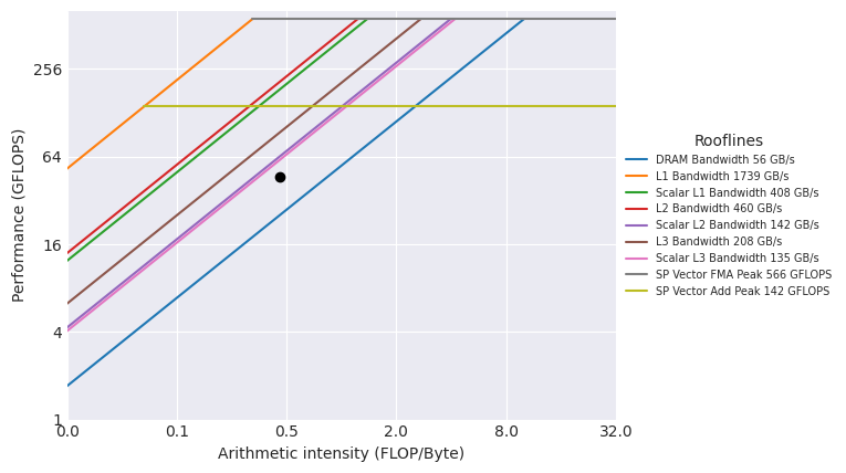
Similarly, we can also produce a graph which displays the most time consuming loop alongside all other loops which have execution time within one order of magnitude from it. This is done by using top-loops mode.
# NBVAL_SKIP
%%bash
python3 $DEVITO_JUPYTER/benchmarks/user/advisor/roofline.py \
    --mode top-loops \
    --name $DEVITO_JUPYTER/examples/performance/resources/TopLoopsRoof \
    --project $DEVITO_JUPYTER/examples/performance/profilings/JupyterProfiling \
Opening project /home/devitouser/devito/examples/performance/profilings/JupyterProfiling... Loading data... Figure saved in /home/devitouser/devito/benchmarks/user/advisor//home/devitouser/devito/examples/performance/resources/TopLoopsRoof.pdf. JSON file saved as /home/devitouser/devito/examples/performance/resources/TopLoopsRoof.json. Done!
With the command having run, we can inspect the image that has been created and compare it to the overview mode roofline.
Image(filename=os.path.join(devito_path, 'examples/performance/resources/TopLoopsRoof.png'))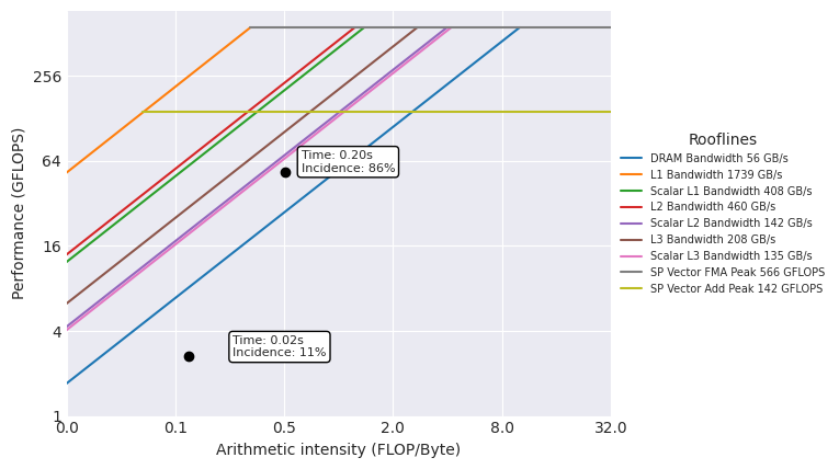
As you can see from this roofline graph, the main point is different from the single point of the previous graph. Moreover, each point is labelled with ‘Time’ and ‘Incidence’ indicators. These represent the total execution time of each loop’s main body and their percentage incidence on the total execution time of the main time loop.
Further flags and functionality
The last two scripts contain more flags that you can use to adjust data collection, displaying and exporting.
roofline.py: * --scale specifies how much rooflines should be scaled down due to using fewer cores than available * --precision specifies the arithmetic precision of the integral operators * --th specifies the threshold percentage over which to display loops in top-loops mode
If you want to learn more about what they do, add a --help flag to the script that you are executing.