import numpy as np
from scipy.special import hankel2
from examples.seismic.acoustic import AcousticWaveSolver
from examples.seismic import Model, AcquisitionGeometry
from devito import set_log_level

import matplotlib.pyplot as plt
%matplotlib inlineVerification
# Switch to error logging so that info is printed but runtime is hidden
from devito import configuration
configuration['log-level'] = 'ERROR'
# Model with fixed time step value
class ModelBench(Model):
"""
Physical model used for accuracy benchmarking.
The critical dt is made small enough to ignore
time discretization errors
"""
@property
def critical_dt(self):
"""Critical computational time step value."""
return .1We compute the error between the numerical and reference solutions for varying spatial discretization order and grid spacing. We also compare the time to solution to the error for these parameters.
# Discretization order
orders = (2, 4, 6, 8, 10)
norder = len(orders)
# Number of time steps
nt = 1501
# Time axis
dt = 0.1
t0 = 0.
tn = dt * (nt-1)
time = np.linspace(t0, tn, nt)
print(f't0, tn, dt, nt; {t0:.4f} {tn:.4f} {dt:.4f} {nt:d}')
# Source peak frequency in KHz
f0 = .09t0, tn, dt, nt; 0.0000 150.0000 0.1000 1501# Domain sizes and gird spacing
shapes = ((201, 2.0), (161, 2.5), (101, 4.0))
dx = [2.0, 2.5, 4.0]
nshapes = len(shapes)# Fine grid model
c0 = 1.5
model = ModelBench(vp=c0, origin=(0., 0.), spacing=(.5, .5), bcs="damp",
shape=(801, 801), space_order=20, nbl=40, dtype=np.float64)# Source and receiver geometries
src_coordinates = np.empty((1, 2))
src_coordinates[0, :] = 200.
# Single receiver offset 100 m from source
rec_coordinates = np.empty((1, 2))
rec_coordinates[:, :] = 260.
print("The computational Grid has ({}, {}) grid points "
"and a physical extent of ({}m, {}m)".format(*model.grid.shape, *model.grid.extent))
print("Source is at the center with coordinates ({}m, {}m)".format(*tuple(src_coordinates[0])))
print("Receiver (single receiver) is located at ({}m, {}m) ".format(*tuple(rec_coordinates[0])))
# Note: gets time sampling from model.critical_dt
geometry = AcquisitionGeometry(model, rec_coordinates, src_coordinates,
t0=t0, tn=tn, src_type='Ricker', f0=f0, t0w=1.5/f0)The computational Grid has (881, 881) grid points and a physical extent of (440.0m, 440.0m)
Source is at the center with coordinates (200.0m, 200.0m)
Receiver (single receiver) is located at (260.0m, 260.0m) Reference solution for numerical convergence
solver = AcousticWaveSolver(model, geometry, kernel='OT2', space_order=8)
ref_rec, ref_u, _ = solver.forward()
Analytical solution for comparison with the reference numerical solution
The analytical solution of the 2D acoustic wave-equation with a source pulse is defined as:
\[ \begin{aligned} u_s(r, t) &= \frac{1}{2\pi} \int_{-\infty}^{\infty} \{ -i \pi H_0^{(2)}\left(k r \right) q(\omega) e^{i\omega t} d\omega\}\\[10pt] r &= \sqrt{(x - x_{src})^2+(y - y_{src})^2} \end{aligned} \]
where \(H_0^{(2)}\) is the Hankel function of the second kind, \(F(\omega)\) is the Fourier spectrum of the source time function at angular frequencies \(\omega\) and \(k = \frac{\omega}{v}\) is the wavenumber.
We look at the analytical and numerical solution at a single grid point. We ensure that this grid point is on-the-grid for all discretizations analysed in the further verification.
# Source and receiver coordinates
sx, sz = src_coordinates[0, :]
rx, rz = rec_coordinates[0, :]


# Define a Ricker wavelet shifted to zero lag for the Fourier transform
def ricker(f, T, dt, t0):
    t = np.linspace(-t0, T-t0, int(T/dt))
    tt = (np.pi**2) * (f**2) * (t**2)
    y = (1.0 - 2.0 * tt) * np.exp(- tt)
    return y


def analytical(nt, model, time, **kwargs):
    dt = kwargs.get('dt', model.critical_dt)
    # Fourier constants
    nf = int(nt/2 + 1)
    # fnyq = 1. / (2 * dt)
    df = 1.0 / time[-1]
    faxis = df * np.arange(nf)

    wavelet = ricker(f0, time[-1], dt, 1.5/f0)

    # Take the Fourier transform of the source time-function
    R = np.fft.fft(wavelet)
    R = R[0:nf]
    nf = len(R)

    # Compute the Hankel function and multiply by the source spectrum
    U_a = np.zeros((nf), dtype=complex)
    for a in range(1, nf-1):
        k = 2 * np.pi * faxis[a] / c0
        tmp = k * np.sqrt(((rx - sx))**2 + (rz - sz)**2)
        U_a[a] = -1j * np.pi * hankel2(0.0, tmp) * R[a]

    # Do inverse fft on 0:dt:T and you have analytical solution
    U_t = 1.0/(2.0 * np.pi) * np.real(np.fft.ifft(U_a[:], nt))

    # The analytic solution needs be scaled by dx^2 to convert to pressure
    return np.real(U_t) * (model.spacing[0]**2)
time1 = np.linspace(0.0, 3000., 30001)
U_t = analytical(30001, model, time1, dt=time1[1] - time1[0])
U_t = U_t[0:1501]# NBVAL_IGNORE_OUTPUT
print(
f'Numerical data min,max,abs; {np.min(ref_rec.data):+.6e} '
f'{np.max(ref_rec.data):+.6e} {np.max(np.abs(ref_rec.data)):+.6e}'
)
print(
f'Analytic data min,max,abs; {np.min(U_t):+.6e} '
f'{np.max(U_t):+.6e} {np.max(np.abs(U_t)):+.6e}'
)Numerical data min,max,abs; -5.349877e-03 +8.529867e-03 +8.529867e-03
Analytic data min,max,abs; -5.322232e-03 +8.543911e-03 +8.543911e-03# NBVAL_IGNORE_OUTPUT
# Plot wavefield and source/rec position
plt.figure(figsize=(8, 8))
amax = np.max(np.abs(ref_u.data[1, :, :]))
plt.imshow(ref_u.data[1, :, :], vmin=-1.0 * amax, vmax=+1.0 * amax, cmap="seismic")
# plot position of the source in model, add nbl for correct position
plt.plot(2*sx+40, 2*sz+40, 'r*', markersize=11, label='source')
# plot position of the receiver in model, add nbl for correct position
plt.plot(2*rx+40, 2*rz+40, 'k^', markersize=8, label='receiver')
plt.legend()
plt.xlabel('x position (m)')
plt.ylabel('z position (m)')
plt.savefig('wavefieldperf.pdf')
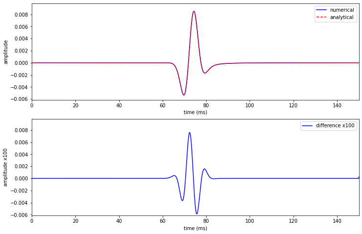
# Plot trace
plt.figure(figsize=(12, 8))
plt.subplot(2, 1, 1)
plt.plot(time, ref_rec.data[:, 0], '-b', label='numerical')
plt.plot(time, U_t[:], '--r', label='analytical')
plt.xlim([0, 150])
plt.ylim([1.15*np.min(U_t[:]), 1.15*np.max(U_t[:])])
plt.xlabel('time (ms)')
plt.ylabel('amplitude')
plt.legend()
plt.subplot(2, 1, 2)
plt.plot(time, 100 *(ref_rec.data[:, 0] - U_t[:]), '-b', label='difference x100')
plt.xlim([0, 150])
plt.ylim([1.15*np.min(U_t[:]), 1.15*np.max(U_t[:])])
plt.xlabel('time (ms)')
plt.ylabel('amplitude x100')
plt.legend()
plt.savefig('ref.pdf')
plt.show()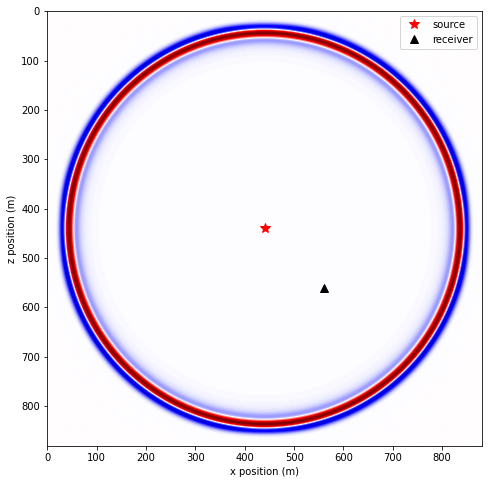
# NBVAL_IGNORE_OUTPUT
error_time = np.zeros(5)
error_time[0] = np.linalg.norm(U_t[:-1] - ref_rec.data[:-1, 0], 2) / np.sqrt(nt)
errors_plot = [(time, U_t[:-1] - ref_rec.data[:-1, 0])]
print(error_time[0])1.1265077536675204e-05Convergence in time
We first show the convergence of the time discretization for a fix high-order spatial discretization (20th order).
After we show that the time discretization converges in \(O(dt^2)\) and therefore only contains the error in time, we will take the numerical solution for dt=.1ms as a reference for the spatial discretization analysis.
# NBVAL_IGNORE_OUTPUT
dt = [0.1000, 0.0800, 0.0750, 0.0625, 0.0500]
nnt = (np.divide(150.0, dt) + 1).astype(int)

for i in range(1, 5):
    # Time axis
    t0 = 0.0
    tn = 150.0
    time = np.linspace(t0, tn, nnt[i])

    # Source geometry
    src_coordinates = np.empty((1, 2))
    src_coordinates[0, :] = 200.

    # Single receiver offset 100 m from source
    rec_coordinates = np.empty((1, 2))
    rec_coordinates[:, :] = 260.

    geometry = AcquisitionGeometry(
        model,
        rec_coordinates,
        src_coordinates,
        t0=t0,
        tn=tn,
        src_type='Ricker',
        f0=f0,
        t0w=1.5/f0
    )

    # Note: incorrect data size will be generated here due to AcquisitionGeometry bug ...
    # temporarily fixed below by resizing the output from the solver
    geometry.resample(dt[i])
    print("geometry.time_axes; ", geometry.time_axis)

    solver = AcousticWaveSolver(model, geometry, time_order=2, space_order=8)
    ref_rec1, ref_u1, _ = solver.forward(dt=dt[i])
    ref_rec1_data = ref_rec1.data[0:nnt[i], :]

    time1 = np.linspace(0.0, 3000., 20*(nnt[i]-1) + 1)
    U_t1 = analytical(20*(nnt[i]-1) + 1, model, time1, dt=time1[1] - time1[0])
    U_t1 = U_t1[0:nnt[i]]

    error_time[i] = np.linalg.norm(U_t1[:-1] - ref_rec1_data[:-1, 0], 2) / np.sqrt(nnt[i]-1)

    ratio_d = dt[i-1]/dt[i] if i > 0 else 1.0
    ratio_e = error_time[i-1]/error_time[i] if i > 0 else 1.0
    print(
        f'error for dt={dt[i]:.4f} is {error_time[i]:12.6e} '
        f'-- ratio dt^2,ratio err; {ratio_d**2:12.6f} {ratio_e:12.6f} \n'
    )
    errors_plot.append((geometry.time_axis.time_values, U_t1[:-1] - ref_rec1_data[:-1, 0]))
geometry.time_axes; TimeAxis: start=0, stop=150.08, step=0.08, num=1877
error for dt=0.0800 is 7.419952e-06 -- ratio dt^2,ratio err; 1.562500 1.518214
geometry.time_axes; TimeAxis: start=0, stop=150, step=0.075, num=2001
error for dt=0.0750 is 6.582594e-06 -- ratio dt^2,ratio err; 1.137778 1.127208
geometry.time_axes; TimeAxis: start=0, stop=150, step=0.0625, num=2401
error for dt=0.0625 is 4.707689e-06 -- ratio dt^2,ratio err; 1.440000 1.398264
geometry.time_axes; TimeAxis: start=0, stop=150, step=0.05, num=3001
error for dt=0.0500 is 3.144849e-06 -- ratio dt^2,ratio err; 1.562500 1.496952
# NBVAL_IGNORE_OUTPUT
plt.figure(figsize=(20, 10))
theory = [t**2 for t in dt]
theory = [error_time[0]*th/theory[0] for th in theory]
plt.loglog([t for t in dt], error_time, '-ob', label=('Numerical'), linewidth=4, markersize=10)
plt.loglog([t for t in dt], theory, '-^r', label=('Theory (2nd order)'), linewidth=4, markersize=10)
for x, y, a in zip([t for t in dt], theory, [(f'dt = {t} ms') for t in dt], strict=True):
    plt.annotate(
        a, xy=(x, y), xytext=(4, 2),
        textcoords='offset points',
        size=20,
        horizontalalignment='left',
        verticalalignment='top'
    )
plt.xlabel("Time-step $dt$ (ms)", fontsize=20)
plt.ylabel("$|| u_{num} - u_{ana}||_2$", fontsize=20)
plt.tick_params(axis='both', which='both', labelsize=20)
plt.tight_layout()
plt.xlim((0.05, 0.1))
plt.legend(fontsize=20, ncol=4, fancybox=True, loc='best')
plt.savefig("TimeConvergence.pdf", format='pdf', facecolor='white',
            orientation='landscape', bbox_inches='tight')
plt.show()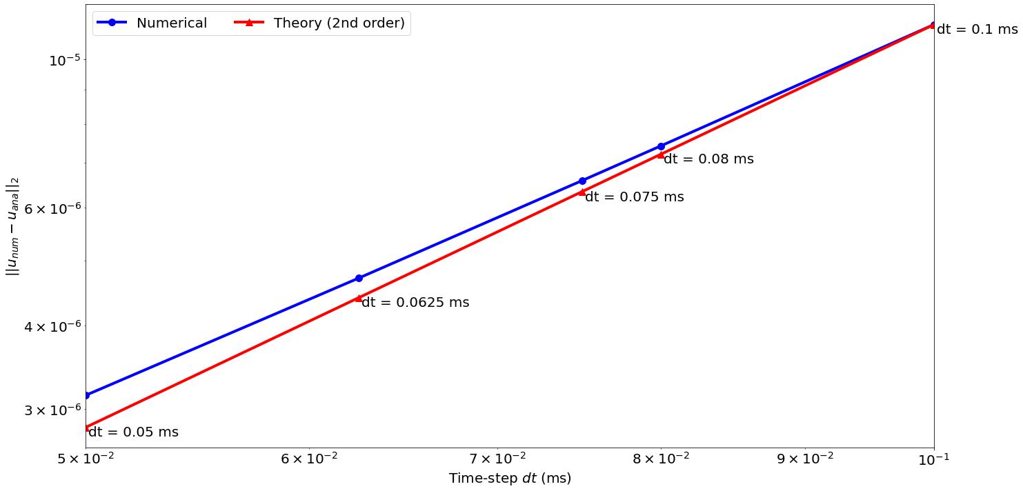
# NBVAL_IGNORE_OUTPUT
stylel = ('--y', '--b', '--r', '--g', '--c')

start_t = lambda dt: int(50/dt)
end_t = lambda dt: int(100/dt)


plt.figure(figsize=(20, 10))

for i, dti in enumerate(dt):
    timei, erri = errors_plot[i]
    s, e = start_t(dti), end_t(dti)
    if i == 0:
        plt.plot(timei[s:e], U_t[s:e], 'k', label='analytical', linewidth=2)
    plt.plot(timei[s:e], 100*erri[s:e], stylel[i], label=f"100 x error dt={dti}ms", linewidth=2)
plt.xlim([50, 100])
plt.xlabel("Time (ms)", fontsize=20)
plt.legend(fontsize=20)
plt.show()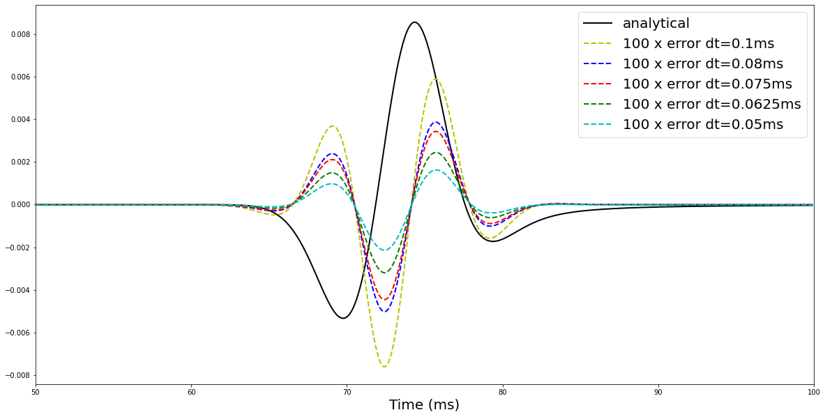
# NBVAL_IGNORE_OUTPUT
pf = np.polyfit(np.log([t for t in dt]), np.log(error_time), deg=1)
print(f"Convergence rate in time is: {pf[0]:.4f}")
assert np.isclose(pf[0], 1.9, atol=0, rtol=.1)
Convergence rate in time is: 1.8403Convergence in space
We have a correct reference solution we can use for space discretization analysis
# NBVAL_IGNORE_OUTPUT
errorl2 = np.zeros((norder, nshapes))
timing = np.zeros((norder, nshapes))

set_log_level("ERROR")
ind_o = -1
for ind_o, spc in enumerate(orders):
    for ind_spc, (nn, h) in enumerate(shapes):
        time = np.linspace(0., 150., nt)

        model_space = ModelBench(vp=c0, origin=(0., 0.), spacing=(h, h), bcs="damp",
                           shape=(nn, nn), space_order=spc, nbl=40, dtype=np.float32)

        # Source geometry
        src_coordinates = np.empty((1, 2))
        src_coordinates[0, :] = 200.

        # Single receiver offset 100 m from source
        rec_coordinates = np.empty((1, 2))
        rec_coordinates[:, :] = 260.

        geometry = AcquisitionGeometry(model_space, rec_coordinates, src_coordinates,
                                       t0=t0, tn=tn, src_type='Ricker', f0=f0, t0w=1.5/f0)

        solver = AcousticWaveSolver(model_space, geometry, time_order=2, space_order=spc)
        loc_rec, loc_u, summary = solver.forward()

        # Note: we need to correct for fixed spacing pressure corrections in both analytic
        # (run at the old model spacing) and numerical (run at the new model spacing) solutions
        c_ana = 1 / model.spacing[0]**2
        c_num = 1 / model_space.spacing[0]**2

        # Compare to reference solution
        # Note: we need to normalize by the factor of grid spacing squared
        errorl2[ind_o, ind_spc] = np.linalg.norm(
            loc_rec.data[:-1, 0] * c_num - U_t[:-1] * c_ana, 2
        ) / np.sqrt(U_t.shape[0] - 1)
        timing[ind_o, ind_spc] = np.max([v for _, v in summary.timings.items()])
        print(
            f'starting space order {spc} with ({nn}, {nn}) grid points the error is '
            f'{errorl2[ind_o, ind_spc]} for {timing[ind_o, ind_spc]} seconds runtime'
        )
starting space order 2 with (201, 201) grid points the error is 0.0037682796393557704 for 0.0457010000000007 seconds runtime
starting space order 2 with (161, 161) grid points the error is 0.005812459176798742 for 0.03416000000000019 seconds runtime
starting space order 2 with (101, 101) grid points the error is 0.013011149171741464 for 0.021772000000000187 seconds runtime
starting space order 4 with (201, 201) grid points the error is 0.0003400355796236851 for 0.05689200000000136 seconds runtime
starting space order 4 with (161, 161) grid points the error is 0.0009414704657502754 for 0.04329800000000062 seconds runtime
starting space order 4 with (101, 101) grid points the error is 0.00634686261474598 for 0.02876700000000098 seconds runtime
starting space order 6 with (201, 201) grid points the error is 4.5490650020112585e-05 for 0.0717499999999997 seconds runtime
starting space order 6 with (161, 161) grid points the error is 0.0002068743812472065 for 0.05577100000000119 seconds runtime
starting space order 6 with (101, 101) grid points the error is 0.003742867493048817 for 0.033743000000000495 seconds runtime
starting space order 8 with (201, 201) grid points the error is 4.1758297084644546e-05 for 0.09771699999999818 seconds runtime
starting space order 8 with (161, 161) grid points the error is 7.16374344942322e-05 for 0.07235899999999956 seconds runtime
starting space order 8 with (101, 101) grid points the error is 0.0025733941924053825 for 0.04383400000000102 seconds runtime
starting space order 10 with (201, 201) grid points the error is 4.4878701635970325e-05 for 0.11604899999999843 seconds runtime
starting space order 10 with (161, 161) grid points the error is 4.998218488476813e-05 for 0.08815700000000024 seconds runtime
starting space order 10 with (101, 101) grid points the error is 0.0019484834503388081 for 0.054120000000001 seconds runtime# NBVAL_IGNORE_OUTPUT
stylel = ('-^k', '-^b', '-^r', '-^g', '-^c')
plt.figure(figsize=(20, 10))
for i in range(0, 5):
plt.loglog(errorl2[i, :], timing[i, :], stylel[i], label=(f'order {orders[i]}'), linewidth=4, markersize=10)
for x, y, a in zip(errorl2[i, :], timing[i, :], [(f'dx = {sc} m') for sc in dx], strict=True):
plt.annotate(
a, xy=(x, y), xytext=(4, 2),
textcoords='offset points', size=20
)
plt.xlabel("$|| u_{num} - u_{ref}||_{inf}$", fontsize=20)
plt.ylabel("Runtime (sec)", fontsize=20)
plt.tick_params(axis='both', which='both', labelsize=20)
plt.tight_layout()
plt.legend(fontsize=20, ncol=3, fancybox=True, loc='lower left')
plt.savefig("TimeAccuracy.pdf", format='pdf', facecolor='white',
orientation='landscape', bbox_inches='tight')
plt.show()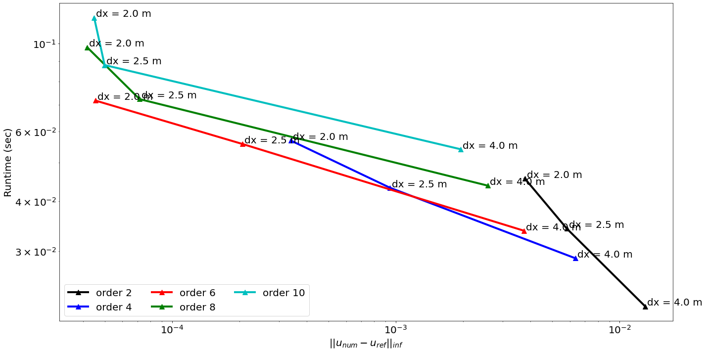
# NBVAL_IGNORE_OUTPUT
stylel = ('-^k', '-^b', '-^r', '-^g', '-^c')
style2 = ('--k', '--b', '--r', '--g', '--c')

plt.figure(figsize=(20, 10))
for i in range(0, 5):
    theory = [k**(orders[i]) for k in dx]
    theory = [errorl2[i, 2]*th/theory[2] for th in theory]
    plt.loglog([sc for sc in dx], errorl2[i, :], stylel[i], label=(f'Numerical order {orders[i]}'),
               linewidth=4, markersize=10)
    plt.loglog([sc for sc in dx], theory, style2[i], label=(f'Theory order {orders[i]}'),
               linewidth=4, markersize=10)
plt.xlabel("Grid spacing $dx$ (m)", fontsize=20)
plt.ylabel("$||u_{num} - u_{ref}||_{inf}$", fontsize=20)
plt.tick_params(axis='both', which='both', labelsize=20)
plt.tight_layout()
plt.legend(fontsize=20, ncol=2, fancybox=True, loc='lower right')
# plt.xlim((2.0, 4.0))
plt.savefig("Convergence.pdf", format='pdf', facecolor='white',
            orientation='landscape', bbox_inches='tight')
plt.show()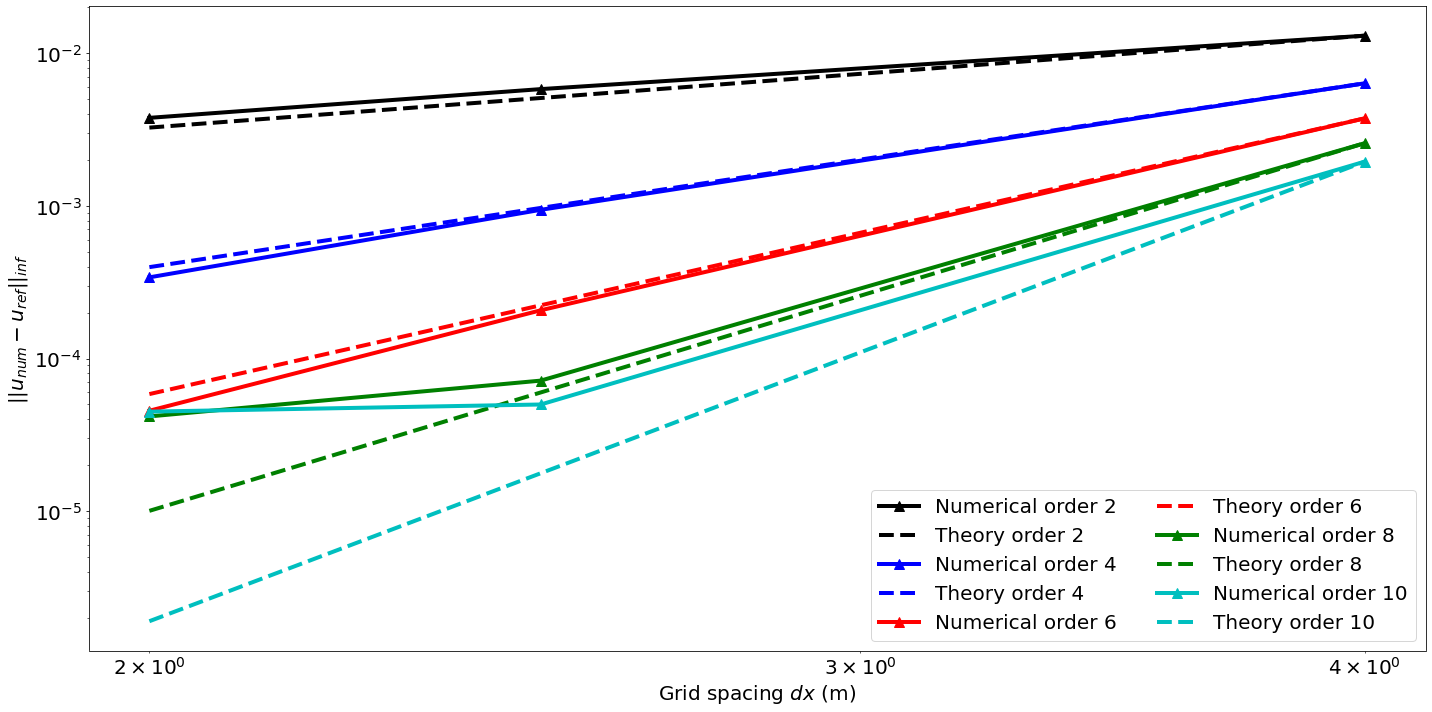
# NBVAL_IGNORE_OUTPUT
for i in range(5):
    pf = np.polyfit(np.log([sc for sc in dx]), np.log(errorl2[i, :]), deg=1)[0]
    if i == 3:
        pf = np.polyfit(np.log([sc for sc in dx][1:]), np.log(errorl2[i, 1:]), deg=1)[0]
    print(f"Convergence rate for order {orders[i]} is {pf}")
    if i < 4:
        assert np.isclose(pf, orders[i], atol=0, rtol=.2)
Convergence rate for order 2 is 1.7764468171576273
Convergence rate for order 4 is 4.197237865060114
Convergence rate for order 6 is 6.331251845625753
Convergence rate for order 8 is 7.619862944985301
Convergence rate for order 10 is 5.803734097693632