import numpy as np
import sympy as sp
from devito import Grid, TimeFunction

# Create our grid (computational domain)
Lx = 10
Ly = Lx
Nx = 11
Ny = Nx
dx = Lx/(Nx-1)
dy = dx
grid = Grid(shape=(Nx, Ny), extent=(Lx, Ly))

# Define u(x,y,t) on this grid
u = TimeFunction(name='u', grid=grid, time_order=2, space_order=2)

# Define symbol for laplacian replacement
H = sp.symbols('H')07 - Custom finite difference coefficients in Devito
Introduction
When taking the numerical derivative of a function in Devito, the default behaviour is for ‘standard’ finite difference weights (obtained via a Taylor series expansion about the point of differentiation) to be applied. Consider the following example for some field \(u(\mathbf{x},t)\), where \(\mathbf{x}=(x,y)\). Let us define a computational domain/grid and differentiate our field with respect to \(x\).
Now, lets look at the output of \(\partial u/\partial x\):
print(u.dx.evaluate)-u(t, x, y)/h_x + u(t, x + h_x, y)/h_xBy default the ‘standard’ Taylor series expansion result, where h_x represents the \(x\)-direction grid spacing, is returned. However, there may be instances when a user wishes to use ‘non-standard’ weights when, for example, implementing a dispersion-relation-preserving (DRP) scheme. See e.g.
[1] Christopher K.W. Tam, Jay C. Webb (1993). ”Dispersion-Relation-Preserving Finite Difference Schemes for Computational Acoustics.” J. Compute. Phys., 107(2), 262–281. https://doi.org/10.1006/jcph.1993.1142
for further details. The use of such modified weights is facilitated in Devito via the custom finite difference coefficients functionality. Lets form a Devito equation featuring a derivative with custom coefficients:
from devito import Eq
weights = np.array([-0.6, 0.1, 0.6])
eq = Eq(u.dt+u.dx(weights=weights))
print(eq.evaluate)
Eq(-u(t, x, y)/dt + u(t + dt, x, y)/dt + 0.1*u(t, x, y)/h_x - 0.6*u(t, x - h_x, y)/h_x + 0.6*u(t, x + h_x, y)/h_x, 0)We see that in the above equation the standard weights for the first derivative of u in the \(x\)-direction have now been replaced with our user defined weights. Note that since custom weights were not specified for the time derivative (u.dt), standard weights are retained.
Now, let us consider a more complete example.
Example: Finite difference modeling for a large velocity-contrast acoustic wave model
It is advised to read through the ‘Introduction to seismic modelling’ notebook located in devito/examples/seismic/tutorials/01_modelling.ipynb before proceeding with this example since much introductory material will be omitted here. The example now considered is based on an example introduced in
[2] Yang Liu (2013). ”Globally optimal finite-difference schemes based on least squares.” GEOPHYSICS, 78(4), 113–132. https://doi.org/10.1190/geo2012-0480.1.
See figure 18 of [2] for further details. Note that here we will simply use Devito to ‘reproduce’ the simulations leading to two results presented in the aforementioned figure. No analysis of the results will be carried out. The domain under consideration has a sptaial extent of \(2km \times 2km\) and, letting \(x\) be the horizontal coordinate and \(z\) the depth, a velocity profile such that \(v_1(x,z)=1500ms^{-1}\) for \(z\leq1200m\) and \(v_2(x,z)=4000ms^{-1}\) for \(z>1200m\).
# NBVAL_IGNORE_OUTPUT
from examples.seismic import Model, plot_velocity
%matplotlib inline

# Define a physical size
Lx = 2000
Lz = Lx
h = 10
Nx = int(Lx/h)+1
Nz = Nx

shape = (Nx, Nz)  # Number of grid point
spacing = (h, h)  # Grid spacing in m. The domain size is now 2km by 2km
origin = (0., 0.)

# Our scheme will be 10th order (or less) in space.
order = 10

# Define a velocity profile. The velocity is in km/s
v = np.empty(shape, dtype=np.float32)
v[:, :121] = 1.5
v[:, 121:] = 4.0

# With the velocity and model size defined, we can create the seismic model that
# encapsulates these properties. We also define the size of the absorbing layer as 10 grid points
nbl = 10
model = Model(vp=v, origin=origin, shape=shape, spacing=spacing,
              space_order=20, nbl=nbl, bcs="damp")

plot_velocity(model)
Operator `initdamp` ran in 0.01 s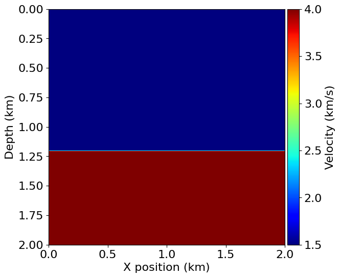
The seismic wave source term will be modelled as a Ricker Wavelet with a peak-frequency of \(25\)Hz located at \((1000m,800m)\). Before applying the DRP scheme, we begin by generating a ‘reference’ solution using a spatially high-order standard finite difference scheme and time step well below the model’s critical time-step. The scheme will be 2nd order in time.
# NBVAL_IGNORE_OUTPUT
from examples.seismic import RickerSource, TimeAxis

t0 = 0.  # Simulation starts a t=0
tn = 500.  # Simulation lasts 0.5 seconds (500 ms)
dt = 1.0  # Time step of 0.2ms

time_range = TimeAxis(start=t0, stop=tn, step=dt)

f0 = 0.025  # Source peak frequency is 25Hz (0.025 kHz)
src = RickerSource(name='src', grid=model.grid, f0=f0,
                   npoint=1, time_range=time_range)

# First, position source centrally in all dimensions, then set depth
src.coordinates.data[0, :] = np.array(model.domain_size) * .5
src.coordinates.data[0, -1] = 800.  # Depth is 800m

# We can plot the time signature to see the wavelet
src.show()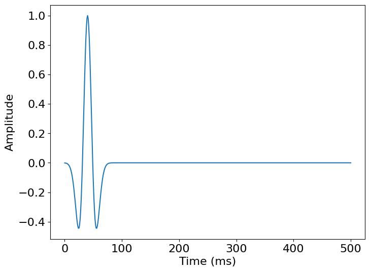
Now let us define our wavefield and PDE:
from devito import solve

# Define the wavefield with the size of the model and the time dimension
u = TimeFunction(name="u", grid=model.grid, time_order=2, space_order=order)

# We can now write the PDE
pde = model.m * u.dt2 - H + model.damp * u.dt

# This discrete PDE can be solved in a time-marching way updating u(t+dt) from the previous time step
# Devito as a shortcut for u(t+dt) which is u.forward. We can then rewrite the PDE as
# a time marching updating equation known as a stencil using customized SymPy functions

stencil = Eq(u.forward, solve(pde, u.forward).subs({H: u.laplace}))
# Finally we define the source injection and receiver read function to generate the corresponding code
src_term = src.inject(field=u.forward, expr=src * dt**2 / model.m)Now, lets create the operator and execute the time marching scheme:
from devito import Operator

op = Operator([stencil] + src_term, subs=model.spacing_map)
# NBVAL_IGNORE_OUTPUT
op(time=time_range.num-1, dt=dt)Operator `Kernel` ran in 0.02 sPerformanceSummary([(PerfKey(name='section0', rank=None),
PerfEntry(time=0.01686700000000005, gflopss=0.0, gpointss=0.0, oi=0.0, ops=0, itershapes=[])),
(PerfKey(name='section1', rank=None),
PerfEntry(time=0.001826, gflopss=0.0, gpointss=0.0, oi=0.0, ops=0, itershapes=[]))])And plot the result:
# NBVAL_IGNORE_OUTPUT
# import matplotlib
import matplotlib.pyplot as plt
from matplotlib import cm
Lx = 2000
Lz = 2000
abs_lay = nbl*h
dx = h
dz = dx
X, Z = np.mgrid[-abs_lay: Lx+abs_lay+1e-10: dx, -abs_lay: Lz+abs_lay+1e-10: dz]
levels = 100
clip = 5
fig = plt.figure(figsize=(14, 7))
ax1 = fig.add_subplot(111)
cont = ax1.imshow(u.data[0, :, :].T, vmin=-clip, vmax=clip, cmap=cm.seismic, extent=[0, Lx, 0, Lz])
fig.colorbar(cont)
ax1.set_xlabel('$x$')
ax1.set_ylabel('$z$')
ax1.set_title('$u(x,z,500)$')
plt.gca().invert_yaxis()
plt.show()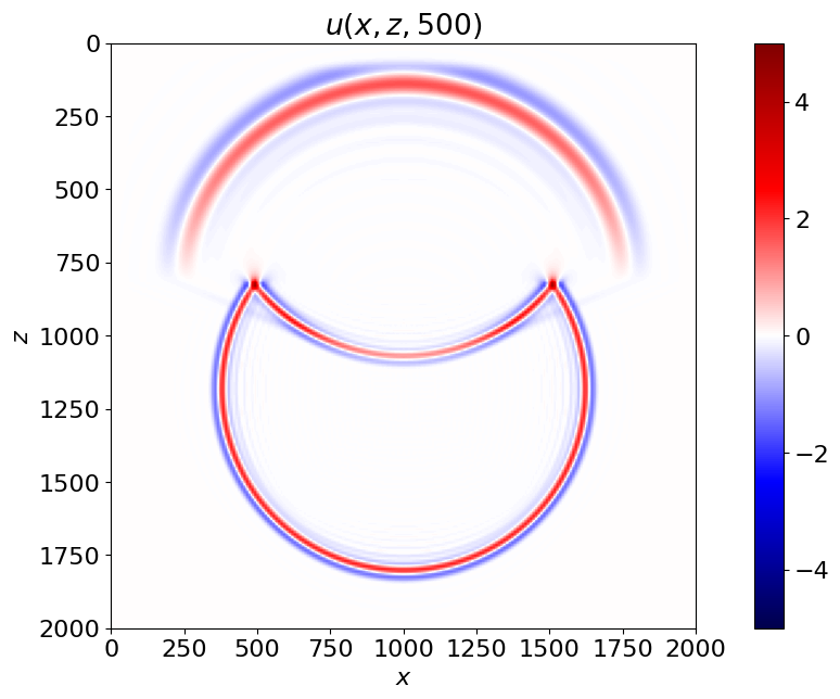
We will now reimplement the above model applying the DRP scheme presented in [2].
First, since we wish to apply different custom FD coefficients in the upper on lower layers we need to define these two ‘subdomains’ using the Devito SubDomain functionality:
from devito import SubDomain
# Define our 'upper' and 'lower' SubDomains:
class Upper(SubDomain):
name = 'upper'
def define(self, dimensions):
x, z = dimensions
# We want our upper layer to span the entire x-dimension and all
# but the bottom 80 (+boundary layer) cells in the z-direction, which is achieved via
# the following notation:
return {x: x, z: ('left', 80+nbl)}
class Lower(SubDomain):
name = 'lower'
def define(self, dimensions):
x, z = dimensions
# We want our lower layer to span the entire x-dimension and all
# but the top 121 (+boundary layer) cells in the z-direction.
return {x: x, z: ('right', 121+nbl)}We now create our Model and attach these SubDomains:
# NBVAL_IGNORE_OUTPUT
# Create our model passing it our 'upper' and 'lower' subdomains:
model = Model(vp=v, origin=origin, shape=shape, spacing=spacing,
space_order=order, nbl=nbl, bcs="damp")
# Create these subdomains:
ur = Upper(grid=model.grid)
lr = Lower(grid=model.grid)Operator `initdamp` ran in 0.01 sAnd re-define model related objects.
t0 = 0. # Simulation starts a t=0
tn = 500. # Simulation last 1 second (500 ms)
dt = 1.0 # Time step of 1.0ms
time_range = TimeAxis(start=t0, stop=tn, step=dt)
f0 = 0.025 # Source peak frequency is 25Hz (0.025 kHz)
src = RickerSource(name='src', grid=model.grid, f0=f0,
npoint=1, time_range=time_range)
src.coordinates.data[0, :] = np.array(model.domain_size) * .5
src.coordinates.data[0, -1] = 800. # Depth is 800m
# New wave-field
u_DRP = TimeFunction(name="u_DRP", grid=model.grid, time_order=2, space_order=order)We now create a stencil for each of our ‘Upper’ and ‘Lower’ subdomains defining different custom FD weights within each of these subdomains. Note that one could shorten the stencil rather than using zero coefficients in the lower layer by providing space_order=order-4 alongside a shorter array of weights.
# The underlying pde is the same in both subdomains
pde_DRP = model.m * u_DRP.dt2 - H + model.damp * u_DRP.dt
# Define our custom FD coefficients:
x, z = model.grid.dimensions
# Upper layer
weights_u = np.array([2.00462e-03, -1.63274e-02, 7.72781e-02,
-3.15476e-01, 1.77768e+00, -3.05033e+00,
1.77768e+00, -3.15476e-01, 7.72781e-02,
-1.63274e-02, 2.00462e-03])
# Lower layer
weights_l = np.array([0., 0., 0.0274017,
-0.223818, 1.64875, -2.90467,
1.64875, -0.223818, 0.0274017,
0., 0.])
# Create the Devito Coefficient objects:
ux_u_coeffs = weights_u/x.spacing**2
uz_u_coeffs = weights_u/z.spacing**2
ux_l_coeffs = weights_l/x.spacing**2
uz_l_coeffs = weights_l/z.spacing**2
u_lap = u_DRP.dx2(weights=ux_u_coeffs) + u_DRP.dy2(weights=uz_u_coeffs)
l_lap = u_DRP.dx2(weights=ux_l_coeffs) + u_DRP.dy2(weights=uz_l_coeffs)
# Create a stencil for each subdomain:
stencil_u = Eq(u_DRP.forward, solve(pde_DRP, u_DRP.forward).subs({H: u_lap}),
subdomain=ur)
stencil_l = Eq(u_DRP.forward, solve(pde_DRP, u_DRP.forward).subs({H: l_lap}),
subdomain=lr)
# Source term:
src_term = src.inject(field=u_DRP.forward, expr=src * dt**2 / model.m)
# Create the operator, incorporating both upper and lower stencils:
op = Operator([stencil_u, stencil_l] + src_term, subs=model.spacing_map)And now execute the operator:
# NBVAL_IGNORE_OUTPUT
op(time=time_range.num-1, dt=dt)
Operator `Kernel` ran in 0.02 sPerformanceSummary([(PerfKey(name='section0', rank=None),
PerfEntry(time=0.015805000000000024, gflopss=0.0, gpointss=0.0, oi=0.0, ops=0, itershapes=[])),
(PerfKey(name='section1', rank=None),
PerfEntry(time=0.0018770000000000076, gflopss=0.0, gpointss=0.0, oi=0.0, ops=0, itershapes=[]))])And plot the new results:
# NBVAL_IGNORE_OUTPUT
fig = plt.figure(figsize=(14, 7))
ax1 = fig.add_subplot(111)
cont = ax1.imshow(u_DRP.data[0, :, :].T, vmin=-clip, vmax=clip, cmap=cm.seismic, extent=[0, Lx, 0, Lz])
fig.colorbar(cont)
ax1.axis([0, Lx, 0, Lz])
ax1.set_xlabel('$x$')
ax1.set_ylabel('$z$')
ax1.set_title('$u_{DRP}(x,z,500)$')

plt.gca().invert_yaxis()
plt.show()
Finally, for comparison, lets plot the difference between the standard 20th order and optimized 10th order models:
# NBVAL_IGNORE_OUTPUT
fig = plt.figure(figsize=(14, 7))
ax1 = fig.add_subplot(111)
cont = ax1.imshow(
    u_DRP.data[0, :, :].T - u.data[0, :, :].T,
    vmin=-clip,
    vmax=clip,
    cmap=cm.seismic,
    extent=[0, Lx, 0, Lz]
)
fig.colorbar(cont)
ax1.set_xlabel('$x$')
ax1.set_ylabel('$z$')

plt.gca().invert_yaxis()
plt.show()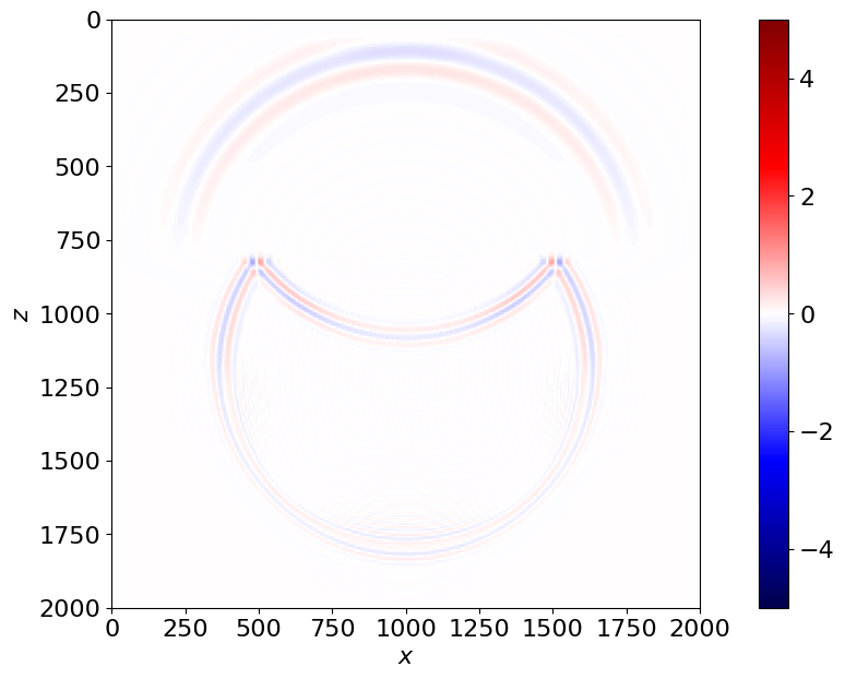
# NBVAL_IGNORE_OUTPUT

# Wavefield norm checks
assert np.isclose(np.linalg.norm(u.data[-1]), 82.170, atol=0, rtol=1e-4)
assert np.isclose(np.linalg.norm(u_DRP.data[-1]), 83.624, atol=0, rtol=1e-4)