from examples.cfd import plot_field, init_hat
import numpy as np
%matplotlib inline

# Some variable declarations
nx = 41  # Grid size on x axis
ny = 41  # Grid size on y axis

batches = 5  # Batches of timesteps, increase number of batches to extend evolution in time
# A figure of the wave state will be produced for each batch.
batch_size = 640  # Number of timesteps for every batch
nt = batches*batch_size  # Number of total timesteps

c = 1
dx = 2. / (nx - 1)
dy = 2. / (ny - 1)
sigma = .0009
nu = 0.01
dt = sigma * dx * dy / nuExample 4: Burgers’ equation
Now that we have seen how to construct the non-linear convection and diffusion examples, we can combine them to form Burgers’ equations. We again create a set of coupled equations which are actually starting to form quite complicated stencil expressions, even if we are only using low-order discretizations.
Let’s start with the definition fo the governing equations: \[ \frac{\partial u}{\partial t} + u \frac{\partial u}{\partial x} + v \frac{\partial u}{\partial y} = \nu \; \left(\frac{\partial ^2 u}{\partial x^2} + \frac{\partial ^2 u}{\partial y^2}\right)\]
\[ \frac{\partial v}{\partial t} + u \frac{\partial v}{\partial x} + v \frac{\partial v}{\partial y} = \nu \; \left(\frac{\partial ^2 v}{\partial x^2} + \frac{\partial ^2 v}{\partial y^2}\right)\]
The discretized and rearranged form then looks like this:
\[\begin{aligned} u_{i,j}^{n+1} &= u_{i,j}^n - \frac{\Delta t}{\Delta x} u_{i,j}^n (u_{i,j}^n - u_{i-1,j}^n) - \frac{\Delta t}{\Delta y} v_{i,j}^n (u_{i,j}^n - u_{i,j-1}^n) \\ &+ \frac{\nu \Delta t}{\Delta x^2}(u_{i+1,j}^n-2u_{i,j}^n+u_{i-1,j}^n) + \frac{\nu \Delta t}{\Delta y^2} (u_{i,j+1}^n - 2u_{i,j}^n + u_{i,j+1}^n) \end{aligned}\] \[\begin{aligned} v_{i,j}^{n+1} &= v_{i,j}^n - \frac{\Delta t}{\Delta x} u_{i,j}^n (v_{i,j}^n - v_{i-1,j}^n) - \frac{\Delta t}{\Delta y} v_{i,j}^n (v_{i,j}^n - v_{i,j-1}^n) \\ &+ \frac{\nu \Delta t}{\Delta x^2}(v_{i+1,j}^n-2v_{i,j}^n+v_{i-1,j}^n) + \frac{\nu \Delta t}{\Delta y^2} (v_{i,j+1}^n - 2v_{i,j}^n + v_{i,j+1}^n) \end{aligned}\]Great. Now before we look at the Devito implementation, let’s re-create the NumPy-based implementation from the original.
# NBVAL_IGNORE_OUTPUT

# Assign initial conditions
u = np.empty((nx, ny))
v = np.empty((nx, ny))

init_hat(field=u, dx=dx, dy=dy, value=2.)
init_hat(field=v, dx=dx, dy=dy, value=2.)

plot_field(u)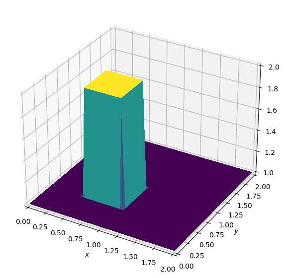
# NBVAL_IGNORE_OUTPUT

for n in range(nt + 1):  # loop across number of time steps
    un = u.copy()
    vn = v.copy()

    u[1:-1, 1:-1] = (un[1:-1, 1:-1] -
                     dt / dy * un[1:-1, 1:-1] *
                     (un[1:-1, 1:-1] - un[1:-1, 0:-2]) -
                     dt / dx * vn[1:-1, 1:-1] *
                     (un[1:-1, 1:-1] - un[0:-2, 1:-1]) +
                     nu * dt / dy**2 *
                     (un[1:-1, 2:] - 2 * un[1:-1, 1:-1] + un[1:-1, 0:-2]) +
                     nu * dt / dx**2 *
                     (un[2:, 1:-1] - 2 * un[1:-1, 1:-1] + un[0:-2, 1:-1]))

    v[1:-1, 1:-1] = (vn[1:-1, 1:-1] -
                     dt / dy * un[1:-1, 1:-1] *
                     (vn[1:-1, 1:-1] - vn[1:-1, 0:-2]) -
                     dt / dx * vn[1:-1, 1:-1] *
                    (vn[1:-1, 1:-1] - vn[0:-2, 1:-1]) +
                     nu * dt / dy**2 *
                     (vn[1:-1, 2:] - 2 * vn[1:-1, 1:-1] + vn[1:-1, 0:-2]) +
                     nu * dt / dx**2 *
                     (vn[2:, 1:-1] - 2 * vn[1:-1, 1:-1] + vn[0:-2, 1:-1]))

    u[0, :] = 1
    u[-1, :] = 1
    u[:, 0] = 1
    u[:, -1] = 1

    v[0, :] = 1
    v[-1, :] = 1
    v[:, 0] = 1
    v[:, -1] = 1

    # A figure of the wave state will be produced for each batch
    if (n % batch_size) == 0:
        print("Batch:", n/(batch_size))
        plot_field(u)
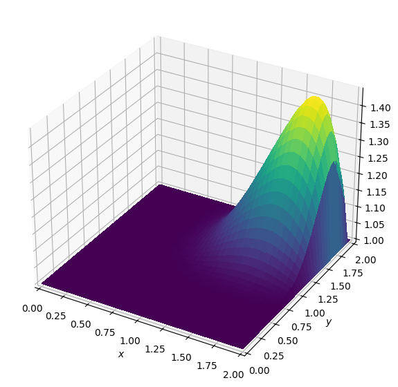
Batch: 0.0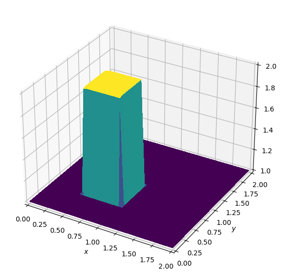
Batch: 1.0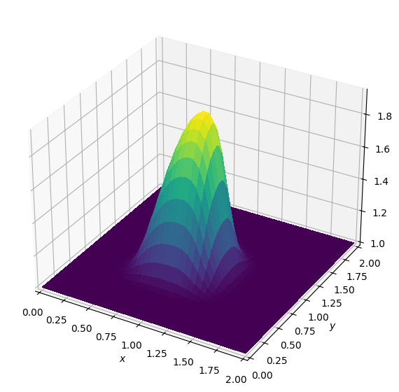
Batch: 2.0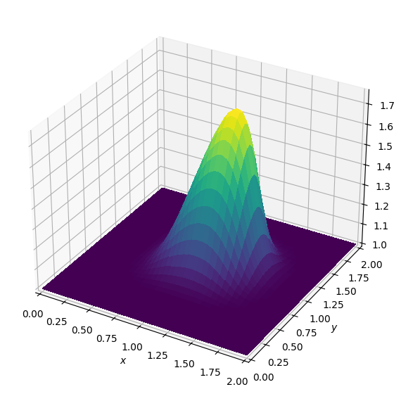
Batch: 3.0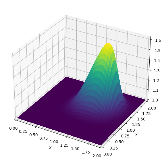
Batch: 4.0
Batch: 5.0
Nice, our wave looks just like the original. Now we shall attempt to write our entire Burgers’ equation operator in a single cell - but before we can demonstrate this, there is one slight problem.
The diffusion term in our equation requires a second-order space discretization on our velocity fields, which we set through the TimeFunction constructor for \(u\) and \(v\). The TimeFunction objects will store this discretisation information and use it as default whenever we use the shorthand notations for derivative, like u.dxl or u.dyl. For the advection term, however, we want to use a first-order discretization, which we now have to create by hand when combining terms with different stencil discretizations. To illustrate let’s consider the following example:
from devito import Grid, TimeFunction, first_derivative, left

grid = Grid(shape=(nx, ny), extent=(2., 2.))
x, y = grid.dimensions
t = grid.stepping_dim

u1 = TimeFunction(name='u1', grid=grid, space_order=1)
print(f"Space order 1:\n{u1.dxl}\n")

u2 = TimeFunction(name='u2', grid=grid, space_order=2)
print(f"Space order 2:\n{u2.dxl}\n")

# We use u2 to create the explicit first-order derivative
u1_dx = first_derivative(u2, dim=x, side=left, fd_order=1)
print(f"Explicit space order 1:\n{u1_dx}\n")
Space order 1:
Derivative(u1(t, x, y), x)
Space order 2:
Derivative(u2(t, x, y), x)
Explicit space order 1:
u2(t, x, y)/h_x - u2(t, x - h_x, y)/h_x
Ok, so by constructing derivative terms explicitly we again have full control of the spatial discretization - the power of symbolic computation. Armed with that trick, we can now build and execute our advection-diffusion operator from scratch in one cell.
# NBVAL_IGNORE_OUTPUT
from devito import Operator, Constant, Eq, solve

# Define our velocity fields and initialize with hat function
u = TimeFunction(name='u', grid=grid, space_order=2)
v = TimeFunction(name='v', grid=grid, space_order=2)
init_hat(field=u.data[0], dx=dx, dy=dy, value=2.)
init_hat(field=v.data[0], dx=dx, dy=dy, value=2.)

# Write down the equations with explicit backward differences
a = Constant(name='a')
u_dx = first_derivative(u, dim=x, side=left, fd_order=1)
u_dy = first_derivative(u, dim=y, side=left, fd_order=1)
v_dx = first_derivative(v, dim=x, side=left, fd_order=1)
v_dy = first_derivative(v, dim=y, side=left, fd_order=1)
eq_u = Eq(u.dt + u*u_dx + v*u_dy, a*u.laplace, subdomain=grid.interior)
eq_v = Eq(v.dt + u*v_dx + v*v_dy, a*v.laplace, subdomain=grid.interior)

# Let SymPy rearrange our stencils to form the update expressions
stencil_u = solve(eq_u, u.forward)
stencil_v = solve(eq_v, v.forward)
update_u = Eq(u.forward, stencil_u)
update_v = Eq(v.forward, stencil_v)

# Create Dirichlet BC expressions using the low-level API
bc_u = [Eq(u[t+1, 0, y], 1.)]  # left
bc_u += [Eq(u[t+1, nx-1, y], 1.)]  # right
bc_u += [Eq(u[t+1, x, ny-1], 1.)]  # top
bc_u += [Eq(u[t+1, x, 0], 1.)]  # bottom
bc_v = [Eq(v[t+1, 0, y], 1.)]  # left
bc_v += [Eq(v[t+1, nx-1, y], 1.)]  # right
bc_v += [Eq(v[t+1, x, ny-1], 1.)]  # top
bc_v += [Eq(v[t+1, x, 0], 1.)]  # bottom

# Create the operator
op = Operator([update_u, update_v] + bc_u + bc_v)

# Execute the operator for a number of timesteps
for batch_no in range(batches):
    op(time=batch_size, dt=dt, a=nu)
    print("Batch:", batch_no+1)
    plot_field(u.data[0])
Operator `Kernel` ran in 0.02 sBatch: 1
Operator `Kernel` ran in 0.02 sBatch: 2
Operator `Kernel` ran in 0.02 sBatch: 3
Operator `Kernel` ran in 0.02 sBatch: 4
Operator `Kernel` ran in 0.02 sBatch: 5
Following the non-linear convection example, we now rewrite this example in term of vectorial equation.
from devito import VectorTimeFunction, grad
x, y = grid.dimensions
# Reinitialise
U = VectorTimeFunction(name='U', grid=grid, space_order=2)
init_hat(field=U[0].data[0], dx=dx, dy=dy, value=2.)
init_hat(field=U[1].data[0], dx=dx, dy=dy, value=2.)

plot_field(U[1].data[0])
Boundary conditions
x, y = grid.dimensions
t = grid.stepping_dim
bc_U = [Eq(U[0][t+1, 0, y], 1.)]  # left
bc_U += [Eq(U[0][t+1, nx-1, y], 1.)]  # right
bc_U += [Eq(U[0][t+1, x, ny-1], 1.)]  # top
bc_U += [Eq(U[0][t+1, x, 0], 1.)]  # bottom
bc_U += [Eq(U[1][t+1, 0, y], 1.)]  # left
bc_U += [Eq(U[1][t+1, nx-1, y], 1.)]  # right
bc_U += [Eq(U[1][t+1, x, ny-1], 1.)]  # top
bc_U += [Eq(U[1][t+1, x, 0], 1.)]  # bottom
Reminder, our equations are thus:
\[ \frac{\partial u}{\partial t} + u \frac{\partial u}{\partial x} + v \frac{\partial u}{\partial y} = \nu \; \left(\frac{\partial ^2 u}{\partial x^2} + \frac{\partial ^2 u}{\partial y^2}\right)\]
\[ \frac{\partial v}{\partial t} + u \frac{\partial v}{\partial x} + v \frac{\partial v}{\partial y} = \nu \; \left(\frac{\partial ^2 v}{\partial x^2} + \frac{\partial ^2 v}{\partial y^2}\right)\]
# Now this is a trivial stencil so let's just write it directly
s = grid.time_dim.spacing
update_U = Eq(U.forward, U - s * (grad(U)*U - a * U.laplace), subdomain=grid.interior)

update_U
\(\displaystyle \left[\begin{matrix}U_x(t + dt, x + h_x/2, y)\\U_y(t + dt, x, y + h_y/2)\end{matrix}\right] = \left[\begin{matrix}- dt \left(- a \left(\frac{\partial^{2}}{\partial x^{2}} U_x(t, x + h_x/2, y) + \frac{\partial^{2}}{\partial y^{2}} U_x(t, x + h_x/2, y)\right) + U_x(t, x + h_x/2, y) \frac{\partial}{\partial x} U_x(t, x + h_x/2, y) + U_y(t, x, y + h_y/2) \frac{\partial}{\partial y} U_x(t, x + h_x/2, y)\right) + U_x(t, x + h_x/2, y)\\- dt \left(- a \left(\frac{\partial^{2}}{\partial x^{2}} U_y(t, x, y + h_y/2) + \frac{\partial^{2}}{\partial y^{2}} U_y(t, x, y + h_y/2)\right) + U_x(t, x + h_x/2, y) \frac{\partial}{\partial x} U_y(t, x, y + h_y/2) + U_y(t, x, y + h_y/2) \frac{\partial}{\partial y} U_y(t, x, y + h_y/2)\right) + U_y(t, x, y + h_y/2)\end{matrix}\right]\)
Inspecting the analytical equations above we can see that we have the update (stencil) as a vectorial equation once again.
We finally run the operator.
# NBVAL_IGNORE_OUTPUT
op = Operator([update_U] + bc_U)
# Execute the operator for a number of timesteps
for batch_no in range(batches):
    op(time=batch_size, dt=dt, a=nu)
    print("Batch:", batch_no+1)
    plot_field(U[0].data[0])
Operator `Kernel` ran in 0.02 sBatch: 1
Operator `Kernel` ran in 0.02 sBatch: 2
Operator `Kernel` ran in 0.02 sBatch: 3
Operator `Kernel` ran in 0.02 sBatch: 4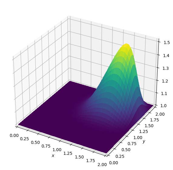
Operator `Kernel` ran in 0.02 sBatch: 5